tidyquant 0.4.0: PerformanceAnalytics, Improved Documentation, ggplot2 Themes and More
Written by Matt Dancho
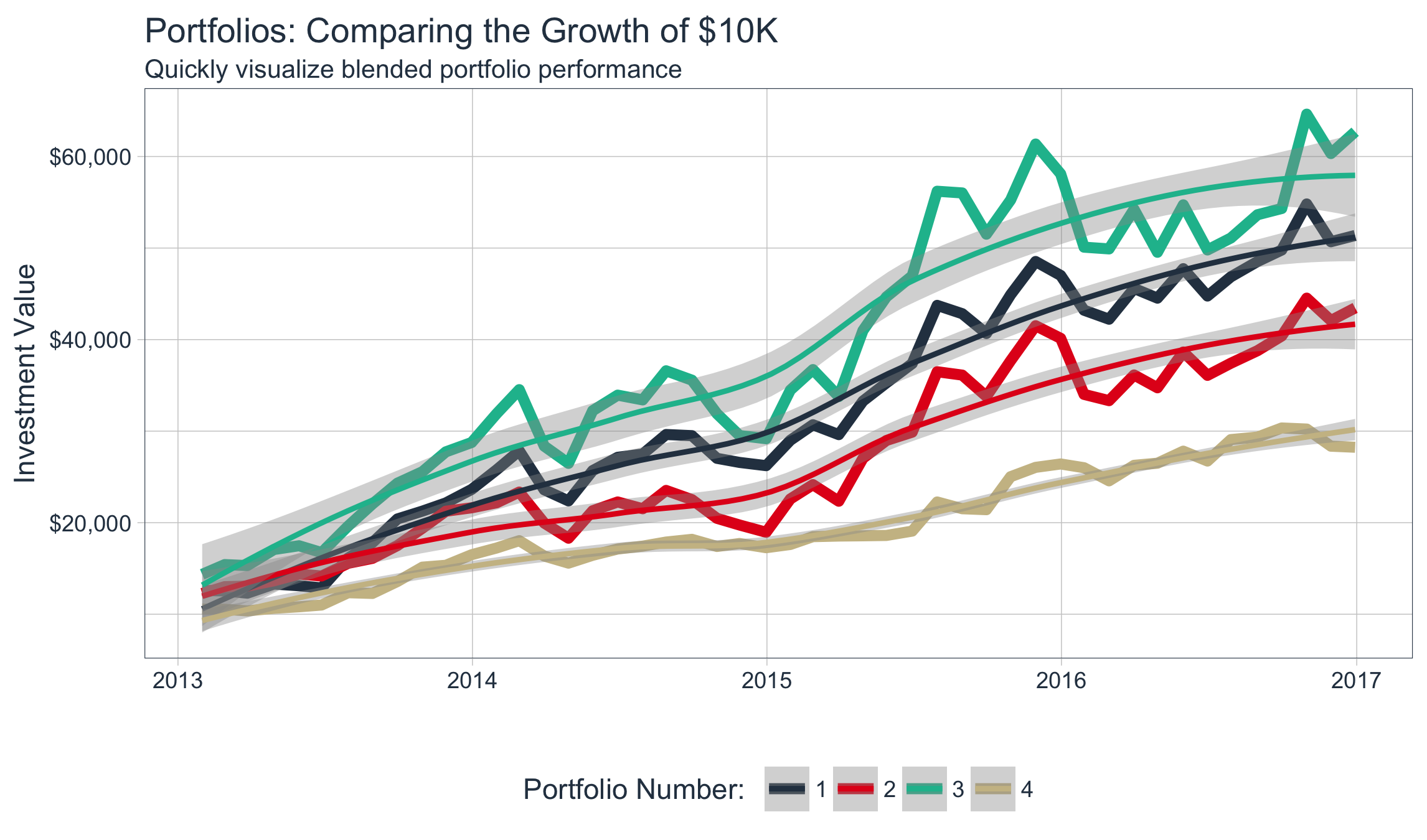
I’m excited to announce the release of tidyquant version 0.4.0!!! The release is yet again sizable. It includes integration with the PerformanceAnalytics package, which now enables full financial analyses to be performed without ever leaving the “tidyverse” (i.e. with DATA FRAMES). The integration includes the ability to perform performance analysis and portfolio attribution at scale (i.e. with many stocks or many portfolios at once)! But wait there’s more… In addition to an introduction vignette, we created five (yes, five!) topic-specific vignettes designed to reduce the learning curve for financial data scientists. We also have new ggplot2 themes to assist with creating beautiful and meaningful financial charts. We included tq_get support for “compound getters” so multiple data sources can be brought into a nested data frame all at once. Last, we have added new tq_index() and tq_exchange() functions to make collecting stock data with tq_get even easier. I’ll briefly touch on several of the updates. The package is open source, and you can view the code on the tidyquant github page.
Table of Contents
Prerequisites
First, update to tidyquant v0.4.0.
install.packages("tidyquant")
Next, load tidyquant.
# Loads tidyquant, tidyverse, lubridate, quantmod, TTR, xts, zoo, PerformanceAnalytics
library(tidyquant)
Load the FANG data set, which will be used in the examples. The FANG data set contains the historical stock prices for FB, AMZN, NFLX, and GOOG from the beginning of 2013 through the end of 2016.
data(FANG)
FANG
## # A tibble: 4,032 × 8
##    symbol       date  open  high   low close    volume adjusted
##     <chr>     <date> <dbl> <dbl> <dbl> <dbl>     <dbl>    <dbl>
## 1      FB 2013-01-02 27.44 28.18 27.42 28.00  69846400    28.00
## 2      FB 2013-01-03 27.88 28.47 27.59 27.77  63140600    27.77
## 3      FB 2013-01-04 28.01 28.93 27.83 28.76  72715400    28.76
## 4      FB 2013-01-07 28.69 29.79 28.65 29.42  83781800    29.42
## 5      FB 2013-01-08 29.51 29.60 28.86 29.06  45871300    29.06
## 6      FB 2013-01-09 29.67 30.60 29.49 30.59 104787700    30.59
## 7      FB 2013-01-10 30.60 31.45 30.28 31.30  95316400    31.30
## 8      FB 2013-01-11 31.28 31.96 31.10 31.72  89598000    31.72
## 9      FB 2013-01-14 32.08 32.21 30.62 30.95  98892800    30.95
## 10     FB 2013-01-15 30.64 31.71 29.88 30.10 173242600    30.10
## # ... with 4,022 more rows
I also recommend the open-source RStudio IDE, which makes R Programming easy and efficient especially for financial analysis.
Overview
tidyquant: Bringing financial analysis to the tidyverse
Before I dive into the updates, if you are new to tidyquant there’s a few core functions that you need to be aware of:
-
Getting Financial Data from the web: tq_get(). This is a one-stop shop for getting web-based financial data in a “tidy” data frame format. Get data for daily stock prices (historical), key statistics (real-time), key ratios (historical), financial statements, dividends, splits, economic data from the FRED, FOREX rates from Oanda.
-
Manipulating Financial Data: tq_transmute() and tq_mutate(). Integration for many financial functions from xts, zoo, quantmod and TTR packages. tq_mutate() is used to add a column to the data frame, and tq_transmute() is used to return a new data frame which is necessary for periodicity changes. Important: In v0.4.0, tq_transmute() replaces tq_transform() for consistency with dplyr::transmute().
-
Coercing Data To and From xts and tibble: as_tibble()and as_xts(). There are a ton of Stack Overflow articles on converting data frames to and from xts. These two functions can be used to answer 99% of these questions.
-
Performance Analysis and Portfolio Analysis: tq_performance() and tq_portfolio(). The newest additions to the tidyquant family integrate PerformanceAnalytics functions. tq_performance() converts investment returns into performance metrics. tq_portfolio() aggregates a group (or multiple groups) of asset returns into one or more portfolios.
To learn more, browse the new and improved vignettes.
v0.4.0 Updates
We’ve got some neat examples to show off the new capabilities:
- PerformanceAnalytics Integration
- New User-Friendly Vignettes
- New ggplot2 Themes
- “Compound Getters” in tq_get
- tq_index and tq_exchange
The PerformanceAnalytics package does two things very well. First, it enables performance analysis of investment returns using a wide variety of metrics that are detailed in the text, “Practical Portfolio Performance Measurement and Attribution” by Carl Bacon. Second, it enables portfolio aggregation, the process of aggregating a weighted group of stocks or investments into a single set of returns. When combined, this functionality enables portfolio attribution, a set of techniques used to explain a portfolio’s performance versus a benchmark.
The next few examples show off some of the basic capability. These examples scratch the surface of the full capability. Below is a figure demonstrating multiple portfolio analysis, which is an advanced topic discussed in the vignette.

The Sharpe ratio is commonly used in finance as a measure of return per unit risk. The larger the value, the better the reward-to-risk trade off. The PerformanceAnalytics package contains a function SharpeRatio (and SharpeRatio.modified) that can be used to quickly calculate from a set of returns. We’ll use tq_performance to calculate the Sharpe ratio in a “tidy” way, using the PerformanceAnalytics integration. Call tq_performance_fun_options() to see a full list of integrated functions. Spoiler alert: there’s 128 functions divided into 14 categories.
tq_performance() allows us to apply SharpeRatio to “tidy” data frames. The tq_performance() function uses Ra and Rb to specify the asset returns and baseline returns, respectively. These values get passed to the performance_fun, which in our case will be SharpeRatio. The ... allows the user to pass additional arguments to the underlying PerformanceAnalytics function. The arguments are shown below.
args(tq_performance)
## function (data, Ra, Rb = NULL, performance_fun, ...)
## NULL
To understand the end goal, we need to analyze the SharpeRatio function. The arguments are displayed below. It contains R a set of returns, Rf the risk-free rate, p the confidence level, and FUN the value of the denominator (default returns Sharpe ratio using all three), and a few other functions that are not used in this example. It’s important to recognize that R in the SharpeRatio() function is specified using asset returns (Ra) in the tq_performance() function. The baseline returns argument (Rb) in the tq_performance() function is not required since the baseline is not required to calculate SharpeRatio. Just keep in mind that you will either see R or the combination of Ra, Rb in the PerformanceAnalytics function arguments, which indicates whether or not Rb is required in tq_performance().
args(SharpeRatio)
## function (R, Rf = 0, p = 0.95, FUN = c("StdDev", "VaR", "ES"),
##     weights = NULL, annualize = FALSE, ...)
## NULL
Now that we understand the function, we can easily begin the task of getting the Sharpe ratios for the “FANG” stocks. It involves three steps:
- Get data with
tq_get (already done since we have FANG loaded). Make sure to group by symbol if the tibble includes prices for multiple stocks.
- Transmute to period returns with
tq_transmute(mutate_fun = periodReturn)
- Calculate Sharpe ratio with
tq_performance(performance_fun = SharpeRatio)
FANG %>%
    group_by(symbol) %>%
    tq_transmute(ohlc_fun   = Ad,
                 mutate_fun = periodReturn,
                 period     = "daily") %>%
    tq_performance(Ra              = daily.returns,
                   Rb              = NULL,
                   performance_fun = SharpeRatio,
                   Rf              = 0,
                   p               = 0.95,
                   FUN             = "StdDev")
## Source: local data frame [4 x 2]
## Groups: symbol [4]
##
##   symbol `StdDevSharpe(Rf=0%,p=95%)`
##    <chr>                       <dbl>
## 1     FB                  0.07439327
## 2   AMZN                  0.06442433
## 3   NFLX                  0.08402702
## 4   GOOG                  0.05825002
It’s very easy to get performance metrics for multiple stocks. Next, we’ll take a look at portfolio performance.
Combining a group of assets into a portfolio is one of the most useful techniques for controlling risk versus reward. The blending of assets naturally diversifies and can reduce downside risk. Further, portfolio attribution is a set of techniques used to analyze a portfolio or set of portfolios against a benchmark. The newest vignette, Performance Analysis with tidyquant, breaks the process into several steps shown in the workflow diagram below.
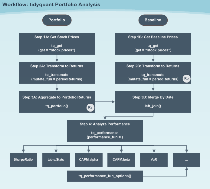
The process for a single portfolio aggregation without a benchmark is shown below. Portfolio aggregation requires a set of weights that can be applied to the various assets (stocks) in the portfolio. Our portfolio consists of FB, AMZN, NFLX, and GOOG. Passing the weights of 50%, 25%, 25%, and 0% blends and aggregates into one set of portfolio returns.
weights <- c(0.50, 0.25, 0.25, 0.00)
FANG_portfolio <- FANG %>%
    group_by(symbol) %>%
    tq_transmute(ohlc_fun   = Ad,
                 mutate_fun = periodReturn,
                 period     = "monthly") %>%
    tq_portfolio(assets_col  = symbol,
                 returns_col = monthly.returns,
                 weights     = weights)
FANG_portfolio
## # A tibble: 48 × 2
##          date portfolio.returns
##        <date>             <dbl>
## 1  2013-01-31       0.260144557
## 2  2013-02-28      -0.004558003
## 3  2013-03-28      -0.019454685
## 4  2013-04-30       0.080958243
## 5  2013-05-31      -0.013883075
## 6  2013-06-28      -0.017906983
## 7  2013-07-31       0.253520291
## 8  2013-08-30       0.103866369
## 9  2013-09-30       0.145446247
## 10 2013-10-31       0.041956895
## # ... with 38 more rows
At this point, it’s nice to visualize using a wealth index, which shows the growth of the portfolio. The wealth index is actually an option in tq_portfolio, but it can also be created by converting the portfolio returns using the cumprod() function shown below.
init.investment <- 10000
FANG_portfolio %>%
    mutate(wealth.index = init.investment * cumprod(1 + portfolio.returns)) %>%
    ggplot(aes(x = date, y = wealth.index)) +
    geom_line(size = 2, color = palette_light()[[3]]) +
    geom_smooth(method = "loess") +
    labs(title = "Individual Portfolio: Comparing the Growth of $10K",
         subtitle = "Quickly visualize performance",
         x = "", y = "Investment Value") +
    theme_tq() +
    scale_y_continuous(labels = scales::dollar)
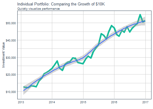
We can even get some performance metrics using PerformanceAnalytics functions. The table functions are the most useful since they calculate groups of portfolio attribution metrics. Eighteen different table functions are available. We’ll use the table.Stats function, which returns a “tidy” set of 15 summary statistics on the stock returns including arithmetic mean, standard deviation, skewness, kurtosis, and more.
FANG_portfolio %>%
    tq_performance(Ra = portfolio.returns,
                   Rb = NULL,
                   performance_fun = table.Stats)
## # A tibble: 1 × 16
##   ArithmeticMean GeometricMean Kurtosis `LCLMean(0.95)` Maximum
## *          <dbl>         <dbl>    <dbl>           <dbl>   <dbl>
## 1         0.0379        0.0347   0.5327          0.0138  0.2601
## # ... with 11 more variables: Median <dbl>, Minimum <dbl>, NAs <dbl>,
## #   Observations <dbl>, Quartile1 <dbl>, Quartile3 <dbl>,
## #   SEMean <dbl>, Skewness <dbl>, Stdev <dbl>, `UCLMean(0.95)` <dbl>,
## #   Variance <dbl>
There’s also capability for performance attribution (comparing portfolio performance against a benchmark) and scaling analyses to multiple portfolios. For those interested in furthering the analysis, please visit the new vignette, Performance Analysis with tidyquant.
2: New User-Friendly Vignettes
Financial analysis can be overwhelming due to the depth and breadth of various topics. Add to it a new package with new functions and workflows, and the task can seem impossible. The good news is we understand.
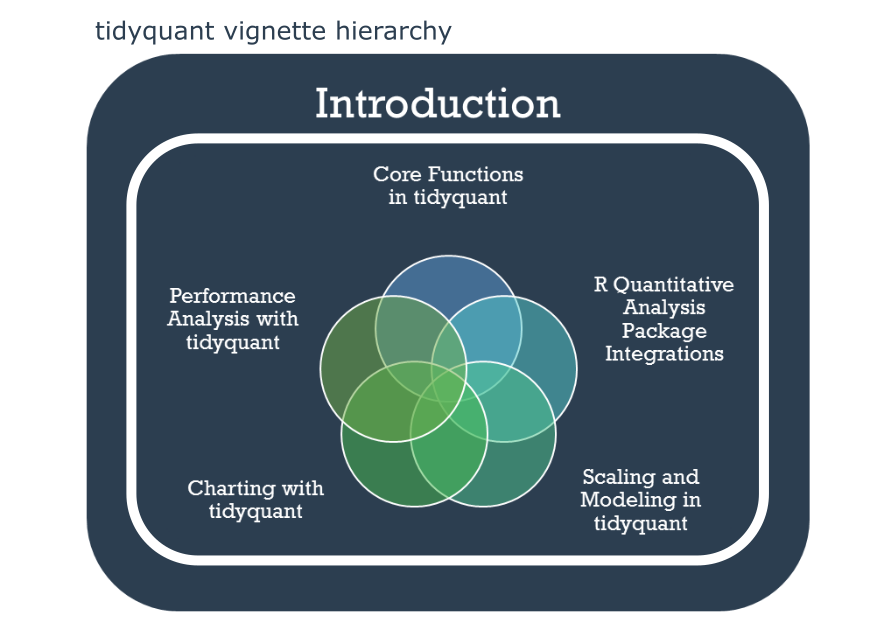
We are actively taking steps to reduce the learning curve so you can get up to speed quickly. While the work is not done yet, we believe that the vignettes are a good place to start. The goal is to break down complex tasks without overloading the user with everything at once. There is now one main “introduction” that links to five topic-specific vignettes. Each topical vignette covers the basics behind the package including real-world examples so you can see how the package can be implemented. You can access the new vignettes here.
3: New ggplot2 Themes
tidyquant ships with some new themes to assist with creating beautiful and meaningful financial charts: theme_tq() and some extra fun ones including theme_tq_dark() and theme_tq_green(). To coordinate aesthetic colors and fills with the appropriate theme, we’ve added scale_color_tq(theme = "light"). You can modify the theme arg to get the colors to correspond with the different themes. In addition, we have palette_light(), palette_dark() and palette_green() for those interested in using the color palette. Here’s a quick example.
FANG %>%
    group_by(symbol) %>%
    tq_transmute(ohlc_fun   = Ad,
                 mutate_fun = periodReturn,
                 period     = "monthly") %>%
    mutate(wealth.index = 10000 * cumprod(1 + monthly.returns)) %>%
    ggplot(aes(x = date, y = wealth.index, color = symbol)) +
    geom_line(size = 1.5) +
    labs(title = "Stocks: Comparing the Growth of $10K",
         subtitle = "New theme for financial visualizations",
         x = "", y = "Investment Value") +
    scale_y_continuous(labels = scales::dollar) +
    theme_tq() +
    scale_color_tq(theme = "light")
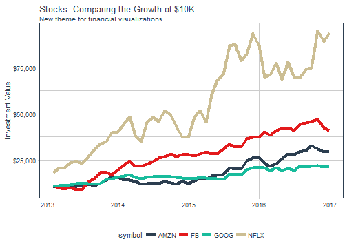
For those interested in learning more about the tidyquant charting capabilities, please visit the updated vignette, Charting with tidyquant.
4: “Compound Getters” in tq_get
Compound getters are a nice tool for those looking to get multiple data sets for one stock symbol. For example, one may want the “key.ratios” and the “key.stats”, which provides key fundamental and financial ratio data on both a historical and real-time basis, respectively. You can now pull this information in one call to tq_get using a “compound getter”.
AAPL_data <- tq_get("AAPL", get = c("key.ratios", "key.stats"))
AAPL_data
## # A tibble: 1 × 3
##   symbol       key.ratios         key.stats
##    <chr>           <list>            <list>
## 1   AAPL <tibble [7 × 2]> <tibble [1 × 55]>
Let’s examine what’s in the “key.ratios” column using unnest().
AAPL_data %>% unnest(key.ratios)
## # A tibble: 7 × 3
##   symbol           section               data
##    <chr>             <chr>             <list>
## 1   AAPL        Financials <tibble [150 × 5]>
## 2   AAPL     Profitability <tibble [170 × 5]>
## 3   AAPL            Growth <tibble [160 × 5]>
## 4   AAPL         Cash Flow  <tibble [50 × 5]>
## 5   AAPL  Financial Health <tibble [240 × 5]>
## 6   AAPL Efficiency Ratios  <tibble [80 × 5]>
## 7   AAPL  Valuation Ratios  <tibble [40 × 5]>
Like peeling away layers we can see whats inside. Let’s do one more unnest.
AAPL_data %>%
    unnest(key.ratios) %>%
    unnest(data)
## # A tibble: 890 × 7
##    symbol    section sub.section group        category       date
##     <chr>      <chr>       <chr> <dbl>           <chr>     <date>
## 1    AAPL Financials  Financials     1 Revenue USD Mil 2007-09-01
## 2    AAPL Financials  Financials     1 Revenue USD Mil 2008-09-01
## 3    AAPL Financials  Financials     1 Revenue USD Mil 2009-09-01
## 4    AAPL Financials  Financials     1 Revenue USD Mil 2010-09-01
## 5    AAPL Financials  Financials     1 Revenue USD Mil 2011-09-01
## 6    AAPL Financials  Financials     1 Revenue USD Mil 2012-09-01
## 7    AAPL Financials  Financials     1 Revenue USD Mil 2013-09-01
## 8    AAPL Financials  Financials     1 Revenue USD Mil 2014-09-01
## 9    AAPL Financials  Financials     1 Revenue USD Mil 2015-09-01
## 10   AAPL Financials  Financials     1 Revenue USD Mil 2016-09-01
## # ... with 880 more rows, and 1 more variables: value <dbl>
We can do the same thing with the “key.stats”. Set .drop = TRUE to remove the “key.ratios” column.
AAPL_data %>% unnest(key.stats, .drop = TRUE)
## # A tibble: 1 × 56
##   symbol    Ask Ask.Size Average.Daily.Volume    Bid Bid.Size
##    <chr>  <dbl>    <dbl>                <dbl>  <dbl>    <dbl>
## 1   AAPL 139.68      200             28964000 139.53      500
## # ... with 50 more variables: Book.Value <dbl>, Change <dbl>,
## #   Change.From.200.day.Moving.Average <dbl>,
## #   Change.From.50.day.Moving.Average <dbl>,
## #   Change.From.52.week.High <dbl>, Change.From.52.week.Low <dbl>,
## #   Change.in.Percent <dbl>, Currency <chr>, Days.High <dbl>,
## #   Days.Low <dbl>, Days.Range <chr>, Dividend.Pay.Date <date>,
## #   Dividend.per.Share <dbl>, Dividend.Yield <dbl>, EBITDA <dbl>,
## #   EPS <dbl>, EPS.Estimate.Current.Year <dbl>,
## #   EPS.Estimate.Next.Quarter <dbl>, EPS.Estimate.Next.Year <dbl>,
## #   Ex.Dividend.Date <date>, Float.Shares <dbl>, High.52.week <dbl>,
## #   Last.Trade.Date <date>, Last.Trade.Price.Only <dbl>,
## #   Last.Trade.Size <dbl>, Last.Trade.With.Time <chr>,
## #   Low.52.week <dbl>, Market.Capitalization <dbl>,
## #   Moving.Average.200.day <dbl>, Moving.Average.50.day <dbl>,
## #   Name <chr>, Open <dbl>, PE.Ratio <dbl>, PEG.Ratio <dbl>,
## #   Percent.Change.From.200.day.Moving.Average <dbl>,
## #   Percent.Change.From.50.day.Moving.Average <dbl>,
## #   Percent.Change.From.52.week.High <dbl>,
## #   Percent.Change.From.52.week.Low <dbl>, Previous.Close <dbl>,
## #   Price.to.Book <dbl>, Price.to.EPS.Estimate.Current.Year <dbl>,
## #   Price.to.EPS.Estimate.Next.Year <dbl>, Price.to.Sales <dbl>,
## #   Range.52.week <chr>, Revenue <dbl>, Shares.Outstanding <dbl>,
## #   Short.Ratio <dbl>, Stock.Exchange <chr>,
## #   Target.Price.1.yr. <dbl>, Volume <dbl>
The benefit to “compound getters” is that all your data is stored in one data frame. To access it, you can simply unnest the list columns. Additionally, the “compound getters” can be scaled in the same way that a single get can be scaled: with a vector of stock symbols or a data frame of stock symbols with the symbols in the first column. See the next section for scaling using the new tq_index() and tq_exchange() functions.
5. tq_index and tq_exchange
We got some really good feedback from a certain someone at RStudio on combining two calls to tq_get() in a row for retrieving an index of stock symbols (e.g. “SP500”) and then the scaling the retrieval of data for the stock symbols. The advice was really good because (1) it was ugly having two calls to tq_get() in a row and (2) more importantly it got us thinking how we can improve scaling data collection. Here’s the significant change from “old way” to the “new way”.
# Not evaluated due to excessive run time
# Old method
tq_get("SP500", get = "stock.index") %>%
    tq_get(get = "stock.prices")

# New method
tq_index("SP500") %>%
    tq_get(get = "stock.prices")
The separation of a stock list from a call to retrieve the data for each of the stocks is fundamentally a good idea because now we can have more lists. For example, if you want to download stock prices for every stock covered on the NASDAQ exchange, you can use the new tq_exchange("NASDAQ") to retrieve the stock list and then pipe (%>%) the list to tq_get.
tq_exchange("NASDAQ")
## # A tibble: 3,169 × 7
##    symbol                                company last.sale.price
##     <chr>                                  <chr>           <dbl>
## 1     PIH 1347 Property Insurance Holdings, Inc.            7.20
## 2    FLWS                1-800 FLOWERS.COM, Inc.            9.85
## 3    FCCY          1st Constitution Bancorp (NJ)           18.65
## 4    SRCE                 1st Source Corporation           47.08
## 5    VNET                   21Vianet Group, Inc.            7.10
## 6    TWOU                               2U, Inc.           37.65
## 7    JOBS                            51job, Inc.           35.60
## 8    CAFD             8point3 Energy Partners LP           12.91
## 9    EGHT                                8x8 Inc           14.90
## 10   AVHI                        A V Homes, Inc.           16.85
## # ... with 3,159 more rows, and 4 more variables: market.cap <chr>,
## #   ipo.year <dbl>, sector <chr>, industry <chr>
Piping to tq_get. (Warning: A word of caution that this could take 10-20 minutes to download the stock prices for all 3169 stock symbols.)
# Not evaluated due to excessive time
tq_exchange("NASDAQ") %>%
    tq_get(get = "stock.prices")
The combination of tq_index and tq_exchange now gives the user access to a wide range of stock lists. To get the full list of options, use tq_index_options() and tq_exchange_options(), respectively.
Conclusions
This is an exciting release for a few reasons. First, the PerformanceAnalytics integration fills a big gap that now allows full financial analysis to be performed within the “tidyverse” (i.e. using data frames only). You can start a workflow with a symbol or set of symbols and through piping (%>%) to tq_get, tq_transmute, and tq_performance can end with performance metrics all in a few lines of code. Previously this was impossible.
Second, portfolio attribution and performance analysis is now possible in the “tidyverse”. This is very interesting because with the data science workflow discussed in R for Data Science the scale at which portfolios can be modeled and analyzed is limitless (refer to many models and the purrr package).
Third, data science is a rapidly evolving field with new people joining the community by the second. With this influx we recognize it’s important to reduce the learning curve for “financial data scientists”, those looking to apply data science to finance. As a result, we are actively taking steps to reduce the learning curve. The first step of providing a set of improved vignettes is complete. We will continue to focus on this area in the future.
Recap
This post was meant to give users and potential users a flavor for the new additions to tidyquant v0.4.0. We took a peek at the new PerformanceAnalytics integration, which enables performance analysis and portfolio aggregation. We introduced the new vignettes, which are topical and are designed to get users up to speed quickly. We discussed several other important new features such as new ggplot2 themes, the new support for “compound getters” in tq_get, and the new tq_index and tq_exchange functions for retrieving stock lists. There are a number of other changes not specifically addressed. Those interested can view the NEWS here.
Further Reading
-
Tidyquant Vignettes: This overview just scratches the surface of tidyquant. The vignettes explain much, much more!
-
R for Data Science: A free book that thoroughly covers the “tidyverse”. A prerequisite for maximizing your abilities with tidyquant.