timekit: New Documentation, Function Improvements, Forecasting Vignette
Written by Matt Dancho

We’ve just released timekit v0.3.0 to CRAN. The package updates include changes that help with making an accurate future time series with tk_make_future_timeseries() and we’ve added a few features to tk_get_timeseries_signature(). Most important are the new vignettes that cover both the making of future time series task and forecasting using the timekit package. If you saw our last timekit post, you were probably surprised to learn that you can use machine learning to forecast using the time series signature as an engineered feature space. Now we are expanding on that concept by providing two new vignettes that teach you how to use ML and data mining for time series predictions. We’re really excited about the prospects of ML applications with time series. If you are too, I strongly encourage you to explore the timekit package important links below. Don’t forget to check out our announcements and to follow us on social media to stay up on the latest Business Science news, events and information! Here’s a summary of the updates.
Updates
We’ve got some great new documentation to really help speed up usage of timekit particularly with respect to applications in forecasting. The doc’s are a big part of the update so we’ll start there first. The package changes have to do with the tk_make_future_timeseries() and tk_get_timeseries_signature() functions. Let’s explore.
New Forecasting Vignette
The vignette Forecasting Using the Time Series Signature with timekit is a new resource for anyone interested in using data mining and machine learning to predict (forecast) future time-based observations. The idea is simple: there’s a lot of information within a time stamp that can be expanded into what is called the time series signature. Patterns between the target and the signature can be modeled or learned. The vignette uses the Bike Sharing Dataset available at the UCI Machine Learning Repository and made popular by Kaggle Competitions. We walk the reader through the forecasting process using the time series signature from start to finish covering all major tasks including:
- Creating training and test sets
- Modeling with the time series signature
- Validating the model using the test set and inspecting the test set accuracy
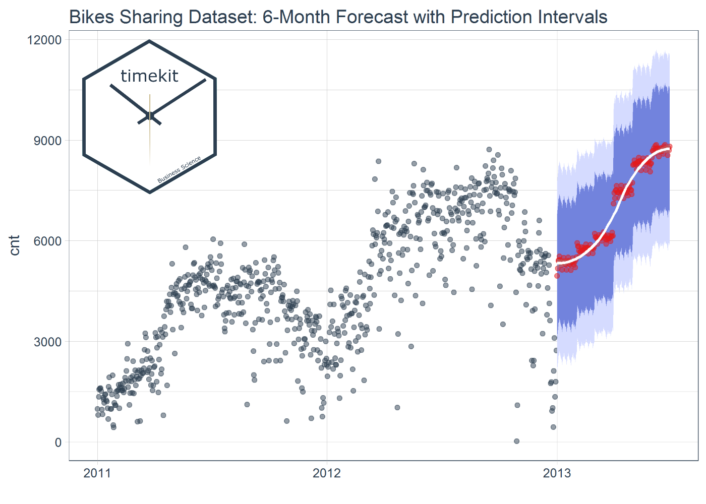
- Forecasting using the model and accounting for prediction intervals
The reader learns how to start with a dataset and end with the forecast shown below!

Check out the Forecasting Vignette!
New Future Time Series Vignette
Making a future time series can be difficult, especially when dealing with daily data that can have missing weekends, holidays, or periods of the year that activity is slower (or non-existent). Further, when forecasting using a time series signature it’s important to get the future time series sequence correct. Fortunately, we’ve put a lot of thought into creating a useful and user friendly function, tk_make_future_timeseries(), to help with this task.
We thought future timeseries accuracy was so important that we gave it a vignette. In the vignette you’ll learn how to inspect a time series to identify patterns in the time series frequency. We show you how to plot the frequency and what to look for. Then, we show you how to use the various arguments to tk_make_future_timeseries() to input the existing index and output a future index that matches your expectations. We focus on the two main arguments that adjust the internal time-series-picking algorithm: inspect_weekdays and inspect_months (new!). We address the pros and cons to each argument by exposing the user to Type I and Type II errors. Then we show how to counteract these errors with skip_values and insert_values (new!). The vignette walks you through the entire process showing you how to create plots to analyze and simulate a future frequency like the one below.

Check out the Future Time Series Index Vignette!
Function Improvements: tk_make_future_timeseries()
The function tk_make_future_timeseries() is a function designed to make your life easier when creating a future time series from an existing one. It evaluates the periodicity of the existing time series and then creates a future time series that matches the frequency. While it works with all frequencies from seconds to years, the biggest benefit is with daily time series.
The tk_make_future_timeseries() function is discussed at length in the vignette so we’ll just go over the changes briefly. To summarize, the function already had the argument inspect_weekdays to look at days that are missing on a weekly, bi-weekly, tri-weekly and quad-weekly frequency. Now it has inspect_months to look for days that are missing on a monthly, quarterly, or yearly schedule. Further, the function already had a skip_values argument to skip irregular time sequences such as holidays. Now it has insert_values to add back in dates that might be incorrectly skipped by the algorithm.
The handling of the n_future argument was changed to now produce an end date that is the number of periods including days removed from inspect_weekends, inspect_months, and skip_days. This helps with keeping a constant end date while varying the inspection and skip days, which is more intuitive when creating a future time series. Here’s a brief example with n_future = 90 using the FB stock from the FANG dataset in the tidyquant package. Note that the end date is always 90 total periods (“2017-03-30”) from the index end date.
library(tidyquant)
library(timekit)

# Get FB stock prices
FB_prices <- FANG %>%
    filter(symbol == "FB") %>%
    select(date, adjusted)

# Extract index
idx <- tk_index(FB_prices)

# Sequential dates matching frequency of idx
idx %>%
    tk_make_future_timeseries(n_future = 90)
##  [1] "2016-12-31" "2017-01-01" "2017-01-02" "2017-01-03" "2017-01-04"
##  [6] "2017-01-05" "2017-01-06" "2017-01-07" "2017-01-08" "2017-01-09"
## [11] "2017-01-10" "2017-01-11" "2017-01-12" "2017-01-13" "2017-01-14"
## [16] "2017-01-15" "2017-01-16" "2017-01-17" "2017-01-18" "2017-01-19"
## [21] "2017-01-20" "2017-01-21" "2017-01-22" "2017-01-23" "2017-01-24"
## [26] "2017-01-25" "2017-01-26" "2017-01-27" "2017-01-28" "2017-01-29"
## [31] "2017-01-30" "2017-01-31" "2017-02-01" "2017-02-02" "2017-02-03"
## [36] "2017-02-04" "2017-02-05" "2017-02-06" "2017-02-07" "2017-02-08"
## [41] "2017-02-09" "2017-02-10" "2017-02-11" "2017-02-12" "2017-02-13"
## [46] "2017-02-14" "2017-02-15" "2017-02-16" "2017-02-17" "2017-02-18"
## [51] "2017-02-19" "2017-02-20" "2017-02-21" "2017-02-22" "2017-02-23"
## [56] "2017-02-24" "2017-02-25" "2017-02-26" "2017-02-27" "2017-02-28"
## [61] "2017-03-01" "2017-03-02" "2017-03-03" "2017-03-04" "2017-03-05"
## [66] "2017-03-06" "2017-03-07" "2017-03-08" "2017-03-09" "2017-03-10"
## [71] "2017-03-11" "2017-03-12" "2017-03-13" "2017-03-14" "2017-03-15"
## [76] "2017-03-16" "2017-03-17" "2017-03-18" "2017-03-19" "2017-03-20"
## [81] "2017-03-21" "2017-03-22" "2017-03-23" "2017-03-24" "2017-03-25"
## [86] "2017-03-26" "2017-03-27" "2017-03-28" "2017-03-29" "2017-03-30"
# Detects and removes weekends that are non-trade days
idx %>%
    tk_make_future_timeseries(n_future = 90, inspect_weekdays = TRUE)
##  [1] "2017-01-02" "2017-01-03" "2017-01-04" "2017-01-05" "2017-01-06"
##  [6] "2017-01-09" "2017-01-10" "2017-01-11" "2017-01-12" "2017-01-13"
## [11] "2017-01-16" "2017-01-17" "2017-01-18" "2017-01-19" "2017-01-20"
## [16] "2017-01-23" "2017-01-24" "2017-01-25" "2017-01-26" "2017-01-27"
## [21] "2017-01-30" "2017-01-31" "2017-02-01" "2017-02-02" "2017-02-03"
## [26] "2017-02-06" "2017-02-07" "2017-02-08" "2017-02-09" "2017-02-10"
## [31] "2017-02-13" "2017-02-14" "2017-02-15" "2017-02-16" "2017-02-17"
## [36] "2017-02-20" "2017-02-21" "2017-02-22" "2017-02-23" "2017-02-24"
## [41] "2017-02-27" "2017-02-28" "2017-03-01" "2017-03-02" "2017-03-03"
## [46] "2017-03-06" "2017-03-07" "2017-03-08" "2017-03-09" "2017-03-10"
## [51] "2017-03-13" "2017-03-14" "2017-03-15" "2017-03-16" "2017-03-17"
## [56] "2017-03-20" "2017-03-21" "2017-03-22" "2017-03-23" "2017-03-24"
## [61] "2017-03-27" "2017-03-28" "2017-03-29" "2017-03-30"
# Manually remove holidays that are irregularly spaced year-to-year
holidays <- ymd("2017-01-02", "2017-01-16", "2017-02-20")
idx %>%
    tk_make_future_timeseries(n_future = 90, inspect_weekdays = TRUE, skip_values = holidays)
##  [1] "2017-01-03" "2017-01-04" "2017-01-05" "2017-01-06" "2017-01-09"
##  [6] "2017-01-10" "2017-01-11" "2017-01-12" "2017-01-13" "2017-01-17"
## [11] "2017-01-18" "2017-01-19" "2017-01-20" "2017-01-23" "2017-01-24"
## [16] "2017-01-25" "2017-01-26" "2017-01-27" "2017-01-30" "2017-01-31"
## [21] "2017-02-01" "2017-02-02" "2017-02-03" "2017-02-06" "2017-02-07"
## [26] "2017-02-08" "2017-02-09" "2017-02-10" "2017-02-13" "2017-02-14"
## [31] "2017-02-15" "2017-02-16" "2017-02-17" "2017-02-21" "2017-02-22"
## [36] "2017-02-23" "2017-02-24" "2017-02-27" "2017-02-28" "2017-03-01"
## [41] "2017-03-02" "2017-03-03" "2017-03-06" "2017-03-07" "2017-03-08"
## [46] "2017-03-09" "2017-03-10" "2017-03-13" "2017-03-14" "2017-03-15"
## [51] "2017-03-16" "2017-03-17" "2017-03-20" "2017-03-21" "2017-03-22"
## [56] "2017-03-23" "2017-03-24" "2017-03-27" "2017-03-28" "2017-03-29"
## [61] "2017-03-30"
Function Improvements: tk_get_timeseries_signature()
We’ve included a few new features that are output when using tk_get_timeseries_signature(). The full list of features can be found on our pkgdown site. The new features include:
- hour12: The hour component on a 12 hour scale.
- am.pm: Morning (AM) = 1, Afternoon (PM) = 2.
- qday: The day of the quarter.
- mweek: The week of the month.
- mday7: The integer division of day of the month by seven. Returns the first, second, third, … instance that the day has appeared in the month. Values begin at 1. For example, the first Saturday in the month has mday7 = 1. The second Saturday has mday7 = 2.
We are now up to 28 features (including the original index) that can be data mined for relationships with the target (response or independent variable).
idx %>%
    tk_get_timeseries_signature()
## # A tibble: 1,008 × 28
##         index  index.num   diff  year  half quarter month month.xts
##        <date>      <int>  <int> <int> <int>   <int> <int>     <int>
## 1  2013-01-02 1357084800     NA  2013     1       1     1         0
## 2  2013-01-03 1357171200  86400  2013     1       1     1         0
## 3  2013-01-04 1357257600  86400  2013     1       1     1         0
## 4  2013-01-07 1357516800 259200  2013     1       1     1         0
## 5  2013-01-08 1357603200  86400  2013     1       1     1         0
## 6  2013-01-09 1357689600  86400  2013     1       1     1         0
## 7  2013-01-10 1357776000  86400  2013     1       1     1         0
## 8  2013-01-11 1357862400  86400  2013     1       1     1         0
## 9  2013-01-14 1358121600 259200  2013     1       1     1         0
## 10 2013-01-15 1358208000  86400  2013     1       1     1         0
## # ... with 998 more rows, and 20 more variables: month.lbl <ord>,
## #   day <int>, hour <int>, minute <int>, second <int>, hour12 <int>,
## #   am.pm <int>, wday <int>, wday.xts <int>, wday.lbl <ord>,
## #   mday <int>, qday <int>, yday <int>, mweek <int>, week <int>,
## #   week.iso <int>, week2 <int>, week3 <int>, week4 <int>,
## #   mday7 <dbl>
Important Links
If you are interested in learning more about timekit:
Announcements
If you’re interested in meeting with the members of Business Science, we’ll be speaking at the following upcoming conferences:
Test