sweep: Extending broom for time series forecasting
Written by Matt Dancho
We’re pleased to introduce a new package, sweep, now on CRAN! Think of it like broom for the forecast package. The forecast package is the most popular package for forecasting, and for good reason: it has a number of sophisticated forecast modeling functions. There’s one problem: forecast is based on the ts system, which makes it difficult work within the tidyverse. This is where sweep fits in! The sweep package has tidiers that convert the output from forecast modeling and forecasting functions to “tidy” data frames. We’ll go through a quick introduction to show how the tidiers can be used, and then show a fun example of forecasting GDP trends of US states. If you’re familiar with broom it will feel like second nature. If you like what you read, don’t forget to follow us on social media to stay up on the latest Business Science news, events and information!
An example of the visualization we can create using sw_sweep() for tidying a forecast:
Benefits
The sweep package makes it easy to transition from the forecast package to the tidyverse. The main benefits are:
-
Converting forecasts to data frames: The forecast package uses ts objects under the hood, thus making it difficult to use in the “tidyverse”. With sw_sweep, we can now easily convert forecasts to tidy data frames.
-
Dates are carried through to the end: The ts objects traditionally lose date information. The sweep package uses timekit under the hood to maintain the original time series index the whole way through the process. The result is ability to forecast in the original date or date-time time-base by setting timekit_idx = TRUE. Future dates are computed using tk_make_future_timeseries() from timekit.
-
Intermediate modeling tidiers: The sweep package uses broom-style tidiers, sw_tidy, sw_glance, and sw_augment to extract important model information into tidy data frames.
Libraries Needed
You can quickly install the packages used with the following script:
# Install packages
pkgs <- c("forecast", "sweep", "timekit", "tidyquant", "geofacet")
install.packages(pkgs)
Load the following packages:
forecast: Has excellent modeling functions such as auto.arima(), ets() and bats() and the forecast() function for predicting future observations.sweep: Tidies the output of forecast functions using a similar strategy as the broom package.timekit: Coercion function tk_ts() for converting a tibble to ts while maintaining time-based data.tidyquant: Used to get FRED data and for its ggplot2 theme.geofacet: Really useful facet_geo() function to visualize facets organized by geography.
# Load packages
library(forecast)   # Most popular forecasting pkg
library(sweep)      # Broom tidiers for forecast pkg
library(timekit)    # Working with time series in R
library(tidyquant)  # Get's data from FRED, loads tidyverse behind the scenes
library(geofacet)   # facet_geo() for visualizing facets organized as states
Data
We’ll be working with Annual Gross Domestic Product (GDP) time series data for each of the US States from the FRED database.
One State: Nebraska
We can get the data for one of the states by using tq_get() from the tidyquant package. The FRED code we will use is “NENGSP”, for Nebraska’s annual GDP. Set get = "economic.data" and supply a date range. By default, the returned values are named “price”. Rename “gdp”.
# Get Annual GDP time series, Nebraska
# https://fred.stlouisfed.org/series/NENGSP
ne_gdp <- tq_get("NENGSP", get = "economic.data", from = "2007-01-01", to = "2017-06-01") %>%
    rename(gdp = price)
ne_gdp
## # A tibble: 10 x 2
##          date    gdp
##        <date>  <int>
##  1 2007-01-01  81926
##  2 2008-01-01  84873
##  3 2009-01-01  86961
##  4 2010-01-01  92231
##  5 2011-01-01  99935
##  6 2012-01-01 101973
##  7 2013-01-01 106765
##  8 2014-01-01 112087
##  9 2015-01-01 113458
## 10 2016-01-01 115345
We’ll need the GDP data for all states to create the GDP by State forecast visualization. Here’s how to get it by scaling with tq_get().
Scaling to All 50 States
The structure of the FRED code begins with the state abbreviation, “NE” for Nebraska, followed by “NGSP”. This means we can pull the data for all states very easily by changing the first two characters.
We start by getting a data frame of state FRED codes and abbreviations. Conveniently, R ships with the state abbreviations stored in state.abb. The mutation just adds “NGSP” to the end of the abbreviation to get the FRED code. It’s really important that the code is in the first column so tq_get can scale the “getter”. The output is stored as states.
# Get codes for all states, make sure FRED code is in first column
states <- tibble(abbreviation = state.abb) %>%
    mutate(fred_code = paste0(abbreviation, "NGSP")) %>%
    select(2:1)
states
## # A tibble: 50 x 2
##    fred_code abbreviation
##        <chr>        <chr>
##  1    ALNGSP           AL
##  2    AKNGSP           AK
##  3    AZNGSP           AZ
##  4    ARNGSP           AR
##  5    CANGSP           CA
##  6    CONGSP           CO
##  7    CTNGSP           CT
##  8    DENGSP           DE
##  9    FLNGSP           FL
## 10    GANGSP           GA
## # ... with 40 more rows
Next, we scale to pull the FRED data for all of the states by simply passing the states data frame to tq_get(). We format the output dropping the “fred_code” column, grouping on “abbreviation”, and renaming the “price” column to “gdp”. The result is stored in states_gdp.
# Scale tq_get to all states
states_gdp <- states %>%
    tq_get(get = "economic.data", from = "2007-01-01", to = "2017-06-01")

# Group and rename
states_gdp <- states_gdp %>%
    select(-fred_code) %>%
    group_by(abbreviation) %>%
    rename(gdp = price)
states_gdp
## # A tibble: 500 x 3
## # Groups:   abbreviation [50]
##    abbreviation       date    gdp
##           <chr>     <date>  <int>
##  1           AL 2007-01-01 169923
##  2           AL 2008-01-01 172646
##  3           AL 2009-01-01 168315
##  4           AL 2010-01-01 174710
##  5           AL 2011-01-01 180665
##  6           AL 2012-01-01 185878
##  7           AL 2013-01-01 190319
##  8           AL 2014-01-01 194404
##  9           AL 2015-01-01 199980
## 10           AL 2016-01-01 204861
## # ... with 490 more rows
We have two data frames now:
Quick Start
We’ll go through the process to show how sweep can help with tidying in the forecast workflow using the Nebraska GDP data, ne_gdp.
Convert to ts
The forecast package works with ts objects so we’ll need to convert from a tibble (tidy data frame). Here’s how using the timekit function, tk_ts(). Supply a start date start = 2017 and frequency freq = 1 for 1 year to setup the ts object. Add silent = TRUE to skip the messages and warnings that the “date” column is being dropped (non-numeric columns are automatically dropped and the user is alerted by default).
# Convert tibble to ts object with tk_ts()
ne_gdp_ts <- ne_gdp %>%
    tk_ts(start = 2017, freq = 1, silent = TRUE)
Model with auto.arima
Now we can model. Let’s use the auto.arima() function from the forecast package. This function is really cool because internally it pre-selects parameters making it easier to get forecasts especially at scale, discussed later. ;)
# Model using auto.arima()
ne_fit_arima <- auto.arima(ne_gdp_ts)
Optional: Apply a modeling tidier
Once we have a model, we can using the sweep tidiers: sw_tidy(), sw_glance and sw_augment. We’ll check out sw_glance to get the model accuracy metrics.
# sw_glance for model accuracy
sw_glance(ne_fit_arima)
## # A tibble: 1 x 12
##                model.desc    sigma    logLik      AIC      BIC
##                     <chr>    <dbl>     <dbl>    <dbl>    <dbl>
## 1 ARIMA(0,1,0) with drift 2149.529 -81.29672 166.5934 166.9879
## # ... with 7 more variables: ME <dbl>, RMSE <dbl>, MAE <dbl>,
## #   MPE <dbl>, MAPE <dbl>, MASE <dbl>, ACF1 <dbl>
Forecast
Next, we create the forecast using the forecast() function from the forecast package. We’ll perform a three year forecast so set h = 3 for 3 periods.
# Three period forecast
ne_fcast <- forecast(ne_fit_arima, h = 3)
Tidy the forecast with sw_sweep
Finally, the beauty of sweep, we can convert the forecast to a tidy data frame.
# Getting a tidy forecast :)
ne_sweep <- sw_sweep(ne_fcast, timekit_idx = TRUE, rename_index = "date")
ne_sweep
## # A tibble: 13 x 7
##          date      key      gdp    lo.80    lo.95    hi.80    hi.95
##        <date>    <chr>    <dbl>    <dbl>    <dbl>    <dbl>    <dbl>
##  1 2007-01-01   actual  81926.0       NA       NA       NA       NA
##  2 2008-01-01   actual  84873.0       NA       NA       NA       NA
##  3 2009-01-01   actual  86961.0       NA       NA       NA       NA
##  4 2010-01-01   actual  92231.0       NA       NA       NA       NA
##  5 2011-01-01   actual  99935.0       NA       NA       NA       NA
##  6 2012-01-01   actual 101973.0       NA       NA       NA       NA
##  7 2013-01-01   actual 106765.0       NA       NA       NA       NA
##  8 2014-01-01   actual 112087.0       NA       NA       NA       NA
##  9 2015-01-01   actual 113458.0       NA       NA       NA       NA
## 10 2016-01-01   actual 115345.0       NA       NA       NA       NA
## 11 2017-01-01 forecast 119058.2 116303.5 114845.2 121813.0 123271.2
## 12 2018-01-01 forecast 122771.4 118875.7 116813.4 126667.2 128729.5
## 13 2019-01-01 forecast 126484.7 121713.3 119187.5 131256.0 133781.8
And, we can easily visualize using ggplot2.
# Visualizing the forecast
ne_sweep %>%
    ggplot(aes(x = date, y = gdp, color = key)) +
    # Prediction intervals
    geom_ribbon(aes(ymin = lo.95, ymax = hi.95),
                fill = "#D5DBFF", color = NA, size = 0) +
    geom_ribbon(aes(ymin = lo.80, ymax = hi.80, fill = key),
                fill = "#596DD5", color = NA, size = 0, alpha = 0.8) +
    # Actual & Forecast
    geom_line(size = 1) +
    geom_point(size = 2) +
    # Aesthetics
    theme_tq(base_size = 16) +
    scale_color_tq() +
    labs(title = "Nebraska GDP, 3-Year Forecast", x = "", y = "GDP, USD Millions")

Now, onto a more sophisticated example.
State GDP Forecasting
Rather than one state, say we wanted to visualize the forecast of the annual GDP for all states so we can get a better understanding of trends. This is now much easier. The general steps are the same, but instead of individually managing each analysis we’ll use purrr to iterate through the 50 states keeping everything “tidy” in the process.
Start with states_gdp, which contains our data for all 50 states. Use nest() to create a nested data frame with the “date” and “gdp” inside a list column.
# Nest the grouped data frame so date and gdp are nested in list columns
states_gdp <- states_gdp %>%
    nest()
states_gdp
## # A tibble: 50 x 2
##    abbreviation              data
##           <chr>            <list>
##  1           AL <tibble [10 x 2]>
##  2           AK <tibble [10 x 2]>
##  3           AZ <tibble [10 x 2]>
##  4           AR <tibble [10 x 2]>
##  5           CA <tibble [10 x 2]>
##  6           CO <tibble [10 x 2]>
##  7           CT <tibble [10 x 2]>
##  8           DE <tibble [10 x 2]>
##  9           FL <tibble [10 x 2]>
## 10           GA <tibble [10 x 2]>
## # ... with 40 more rows
Next, use map() to iteratively apply the tk_ts() function. Add the additional arguments freq = 1, start = 2007 and silent = TRUE. The new column, “data_ts”, contains the data converted ts.
states_gdp <- states_gdp %>%
    mutate(data_ts = map(data, tk_ts, freq = 1, start = 2007, silent = TRUE))
states_gdp
## # A tibble: 50 x 3
##    abbreviation              data  data_ts
##           <chr>            <list>   <list>
##  1           AL <tibble [10 x 2]> <S3: ts>
##  2           AK <tibble [10 x 2]> <S3: ts>
##  3           AZ <tibble [10 x 2]> <S3: ts>
##  4           AR <tibble [10 x 2]> <S3: ts>
##  5           CA <tibble [10 x 2]> <S3: ts>
##  6           CO <tibble [10 x 2]> <S3: ts>
##  7           CT <tibble [10 x 2]> <S3: ts>
##  8           DE <tibble [10 x 2]> <S3: ts>
##  9           FL <tibble [10 x 2]> <S3: ts>
## 10           GA <tibble [10 x 2]> <S3: ts>
## # ... with 40 more rows
Third, use map() again, this time applying the auto.arima function. We can see that a new column is added called fit.
states_gdp <- states_gdp %>%
    mutate(fit = map(data_ts, auto.arima))
states_gdp
## # A tibble: 50 x 4
##    abbreviation              data  data_ts         fit
##           <chr>            <list>   <list>      <list>
##  1           AL <tibble [10 x 2]> <S3: ts> <S3: ARIMA>
##  2           AK <tibble [10 x 2]> <S3: ts> <S3: ARIMA>
##  3           AZ <tibble [10 x 2]> <S3: ts> <S3: ARIMA>
##  4           AR <tibble [10 x 2]> <S3: ts> <S3: ARIMA>
##  5           CA <tibble [10 x 2]> <S3: ts> <S3: ARIMA>
##  6           CO <tibble [10 x 2]> <S3: ts> <S3: ARIMA>
##  7           CT <tibble [10 x 2]> <S3: ts> <S3: ARIMA>
##  8           DE <tibble [10 x 2]> <S3: ts> <S3: ARIMA>
##  9           FL <tibble [10 x 2]> <S3: ts> <S3: ARIMA>
## 10           GA <tibble [10 x 2]> <S3: ts> <S3: ARIMA>
## # ... with 40 more rows
Optionally, we can run glance to get the model accuracies.
states_gdp %>%
    mutate(glance = map(fit, sw_glance)) %>%
    unnest(glance, .drop = T)
## # A tibble: 50 x 13
##    abbreviation                      model.desc     sigma    logLik
##           <chr>                           <chr>     <dbl>     <dbl>
##  1           AL         ARIMA(0,1,0) with drift  3267.828 -85.06590
##  2           AK ARIMA(0,0,0) with non-zero mean  4199.313 -97.08934
##  3           AZ                    ARIMA(0,2,0)  7559.654 -82.79488
##  4           AR         ARIMA(0,1,0) with drift  2231.839 -81.63464
##  5           CA                    ARIMA(0,2,0) 60035.965 -99.37208
##  6           CO         ARIMA(0,1,0) with drift  7064.218 -92.00497
##  7           CT                    ARIMA(0,2,0)  5009.932 -79.50274
##  8           DE         ARIMA(0,1,0) with drift  1865.871 -80.02328
##  9           FL                    ARIMA(0,2,0) 17001.163 -89.27758
## 10           GA                    ARIMA(0,2,0)  6369.686 -81.42147
## # ... with 40 more rows, and 9 more variables: AIC <dbl>, BIC <dbl>,
## #   ME <dbl>, RMSE <dbl>, MAE <dbl>, MPE <dbl>, MAPE <dbl>,
## #   MASE <dbl>, ACF1 <dbl>
Fourth, use map() to apply the forecast function, passing h = 3 as an additional argument.
states_gdp <- states_gdp %>%
    mutate(forecast = map(fit, forecast, h = 3))
states_gdp
## # A tibble: 50 x 5
##    abbreviation              data  data_ts         fit       forecast
##           <chr>            <list>   <list>      <list>         <list>
##  1           AL <tibble [10 x 2]> <S3: ts> <S3: ARIMA> <S3: forecast>
##  2           AK <tibble [10 x 2]> <S3: ts> <S3: ARIMA> <S3: forecast>
##  3           AZ <tibble [10 x 2]> <S3: ts> <S3: ARIMA> <S3: forecast>
##  4           AR <tibble [10 x 2]> <S3: ts> <S3: ARIMA> <S3: forecast>
##  5           CA <tibble [10 x 2]> <S3: ts> <S3: ARIMA> <S3: forecast>
##  6           CO <tibble [10 x 2]> <S3: ts> <S3: ARIMA> <S3: forecast>
##  7           CT <tibble [10 x 2]> <S3: ts> <S3: ARIMA> <S3: forecast>
##  8           DE <tibble [10 x 2]> <S3: ts> <S3: ARIMA> <S3: forecast>
##  9           FL <tibble [10 x 2]> <S3: ts> <S3: ARIMA> <S3: forecast>
## 10           GA <tibble [10 x 2]> <S3: ts> <S3: ARIMA> <S3: forecast>
## # ... with 40 more rows
Finally, use map() to apply the sw_sweep function, passing timekit_idx = TRUE (this gets dates instead of numbers) and rename_index = "date". We no longer need the other columns so select “abbreviation” and “sweep” columns and unnest(). Viola, we have a nice tidy data frame of all of the state forecasts!
states_gdp_sweep <- states_gdp %>%
    mutate(sweep = map(forecast, sw_sweep, timekit_idx = T, rename_index = "date")) %>%
    select(abbreviation, sweep) %>%
    unnest()
states_gdp_sweep
## # A tibble: 650 x 8
##    abbreviation       date    key    gdp lo.80 lo.95 hi.80 hi.95
##           <chr>     <date>  <chr>  <dbl> <dbl> <dbl> <dbl> <dbl>
##  1           AL 2007-01-01 actual 169923    NA    NA    NA    NA
##  2           AL 2008-01-01 actual 172646    NA    NA    NA    NA
##  3           AL 2009-01-01 actual 168315    NA    NA    NA    NA
##  4           AL 2010-01-01 actual 174710    NA    NA    NA    NA
##  5           AL 2011-01-01 actual 180665    NA    NA    NA    NA
##  6           AL 2012-01-01 actual 185878    NA    NA    NA    NA
##  7           AL 2013-01-01 actual 190319    NA    NA    NA    NA
##  8           AL 2014-01-01 actual 194404    NA    NA    NA    NA
##  9           AL 2015-01-01 actual 199980    NA    NA    NA    NA
## 10           AL 2016-01-01 actual 204861    NA    NA    NA    NA
## # ... with 640 more rows
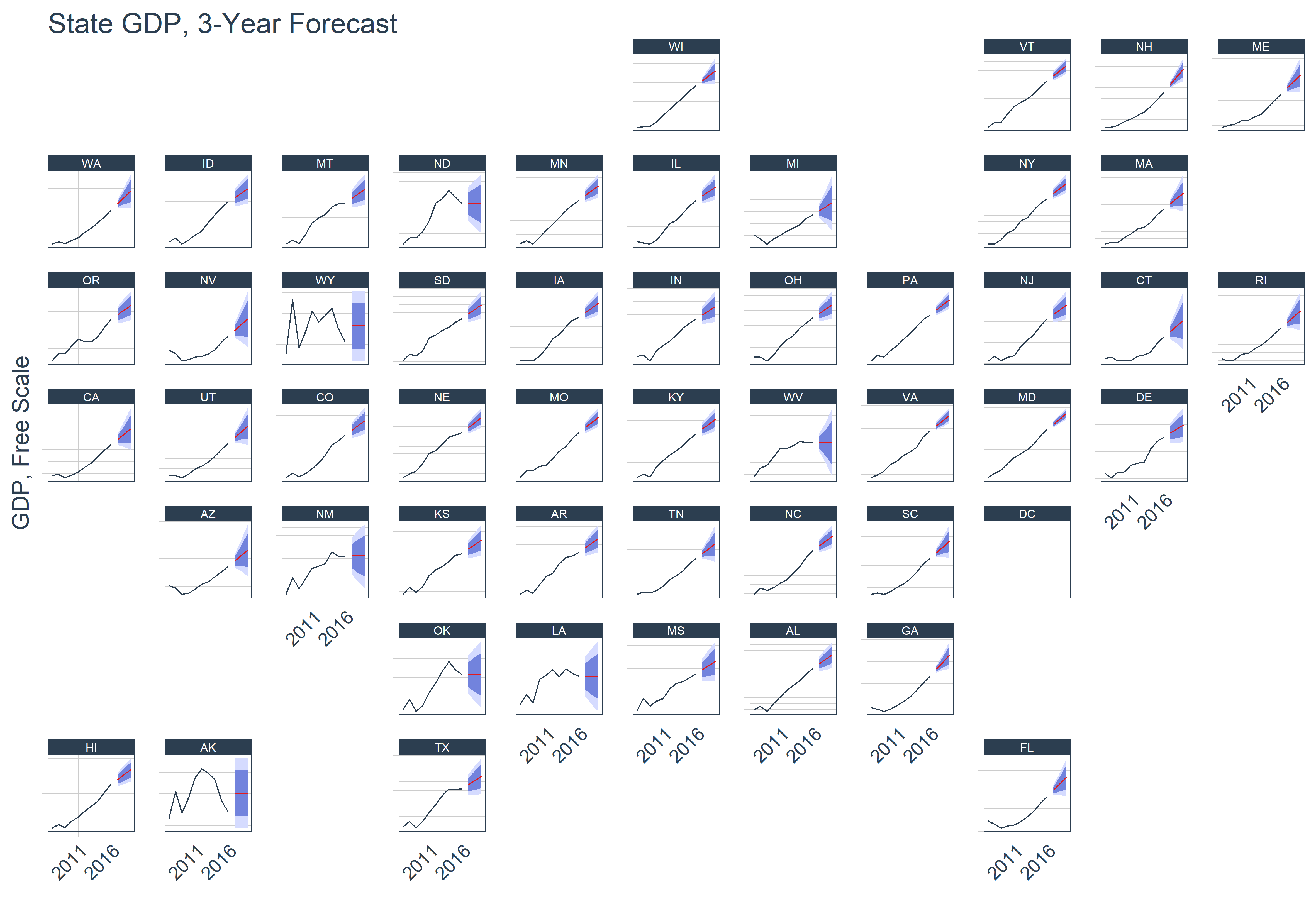
As an added bonus, we can use the facet_geo() function from the geofacet package to visualize the trend and forecast for each state. From the output it looks like most of the states are increasing, but there’s a few with more volatile trends. It might be interesting to investigate what’s causing the deviations in the midwest and south. Possibly related to the recent recession in oil and gas?
# Geofacet
states_gdp_sweep %>%
    ggplot(aes(x = date, y = gdp, color = key)) +
    # Prediction intervals
    geom_ribbon(aes(ymin = lo.95, ymax = hi.95),
                fill = "#D5DBFF", color = NA, size = 0) +
    geom_ribbon(aes(ymin = lo.80, ymax = hi.80, fill = key),
                fill = "#596DD5", color = NA, size = 0, alpha = 0.8) +
    # Actual & Forecast
    geom_line() +
    # Aesthetics
    scale_y_continuous(label = function(x) x*1e-6) +
    scale_x_date(date_breaks = "5 years", labels = scales::date_format("%Y")) +
    facet_geo(~ abbreviation, scale = "free_y") +
    theme_tq() +
    scale_color_tq() +
    theme(legend.position = "none",
          axis.text.x = element_text(angle = 45, hjust = 1),
          axis.text.y = element_blank()
          ) +
    ggtitle("State GDP, 3-Year Forecast") +
    xlab("") +
    ylab("GDP, Free Scale")
Conclusions
The sweep package is a great way to “tidy” the forecast package. It has several functions that tidy model output (sw_tidy, sw_glance, and sw_augment) and forecast output (sw_sweep). A big advantage is that the dates can be kept through the entire process since sweep uses timekit under the hood. If you use the forecast package and love the tidyverse, give sweep a try!
About Business Science
We have a full suite of data science services to supercharge your financial and business performance. How do we do it? Using our network of data science consultants, we pull together the right team to get custom projects done on time, within budget, and of the highest quality. Find out more about our data science services or contact us!
We are growing! Let us know if you are interested in joining our network of data scientist consultants. If you have expertise in Marketing Analytics, Data Science for Business, Financial Analytics, or Data Science in general, we’d love to talk. Contact us!