The Tidy Time Series Platform: tibbletime 0.1.0
Written by Davis Vaughan

We’re happy to announce the third release of the tibbletime package. This is a huge update, mainly due to a complete rewrite of the package. It contains a ton of new functionality and a number of breaking changes that existing users need to be aware of. All of the changes have been well documented in the NEWS file, but it’s worthwhile to touch on a few of them here and discuss the future of the package. We’re super excited so let’s check out the vision for tibbletime and its new functionality!
About Tibbletime
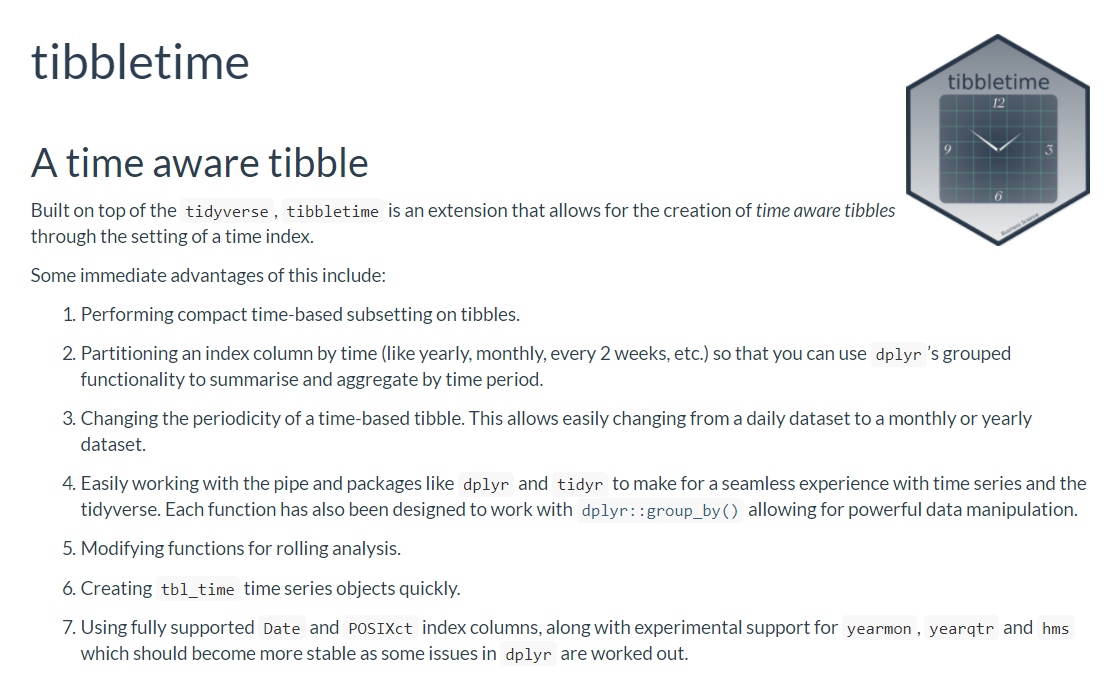
For those new to to package, tibbletime is a new package that enables the creation of time aware tibbles. It’s sole purpose is to make working with time series in the tidyverse much easier! The documentation really explains everything, and here are a few important vignettes that can help get you up to speed on all of the functionality:

Package roadmap
The grand view is to have tibbletime function as a base package that others can build off of, utilizing the infrastructure that “knows” about the index column and provides support for time series transformations on tibbles. This can include extensions to finance, but also has room to grow into other areas such as economic forecasting, longitudinal studies, and other general time series analyses. We’ve already begun work on one such package, but that will be a post for another time ;).
At this point, the first bit of core functionality for tibbletime is complete. A few other functions will likely be added, but we will definitely support backwards compatability from here on out.
New time series capabilities
The tibbletime package was completely re-invisioned, making it much more flexible and general. Here are a few of the important new tools in tibbletime’s toolkit:
-
A new index partitioning function (collapse_index()) that opens up powerful time based analysis with any dplyr function, rather than a specific (and limited) set of time_summarise(), time_mutate(), etc, functions.
-
Full support for Date and POSIXct classes as indices, and experimental support for yearmon, yearqtr, and hms which should get more stable over time.
-
A consistent API along with more informative argument names that attempt to give it that intuitive look and feel of a tidyverse package.
The one downside is that we had to make a few breaking changes, but with this post you’ll be able to easily get your code up to speed with the new functionality. What follows are a few of the most important changes for those that already used tibbletime and are interested in seeing what has changed.
Libraries
Load the following libraries to follow along.
library(tibbletime)
library(dplyr)
time_collapse() -> collapse_index()
Rather than having a function like time_collapse() that worked on an entire tbl_time object, it has been replaced with partition_index() and collapse_index() that solely manipulate the index (date) vector. This allows them to be used inside of a call to mutate() and gives the user more control over the outcome (for example, whether they want to assign it to a new column or overwrite the original index column).
data(FB)

FB_time <- FB %>%
  as_tbl_time(date)

FB_time
## # A time tibble: 1,008 x 8
## # Index: date
##    symbol date        open  high   low close    volume adjusted
##    <chr>  <date>     <dbl> <dbl> <dbl> <dbl>     <dbl>    <dbl>
##  1 FB     2013-01-02  27.4  28.2  27.4  28.0  69846400     28.0
##  2 FB     2013-01-03  27.9  28.5  27.6  27.8  63140600     27.8
##  3 FB     2013-01-04  28.0  28.9  27.8  28.8  72715400     28.8
##  4 FB     2013-01-07  28.7  29.8  28.6  29.4  83781800     29.4
##  5 FB     2013-01-08  29.5  29.6  28.9  29.1  45871300     29.1
##  6 FB     2013-01-09  29.7  30.6  29.5  30.6 104787700     30.6
##  7 FB     2013-01-10  30.6  31.5  30.3  31.3  95316400     31.3
##  8 FB     2013-01-11  31.3  32.0  31.1  31.7  89598000     31.7
##  9 FB     2013-01-14  32.1  32.2  30.6  31.0  98892800     31.0
## 10 FB     2013-01-15  30.6  31.7  29.9  30.1 173242600     30.1
## # ... with 998 more rows
The index has been collapsed. We can now do easy dplyr operations like summarizes.
FB_collapsed <- FB_time %>%
  mutate(date = collapse_index(date, "5 day"))

FB_collapsed
## # A time tibble: 1,008 x 8
## # Index: date
##    symbol date        open  high   low close    volume adjusted
##    <chr>  <date>     <dbl> <dbl> <dbl> <dbl>     <dbl>    <dbl>
##  1 FB     2013-01-04  27.4  28.2  27.4  28.0  69846400     28.0
##  2 FB     2013-01-04  27.9  28.5  27.6  27.8  63140600     27.8
##  3 FB     2013-01-04  28.0  28.9  27.8  28.8  72715400     28.8
##  4 FB     2013-01-11  28.7  29.8  28.6  29.4  83781800     29.4
##  5 FB     2013-01-11  29.5  29.6  28.9  29.1  45871300     29.1
##  6 FB     2013-01-11  29.7  30.6  29.5  30.6 104787700     30.6
##  7 FB     2013-01-11  30.6  31.5  30.3  31.3  95316400     31.3
##  8 FB     2013-01-11  31.3  32.0  31.1  31.7  89598000     31.7
##  9 FB     2013-01-16  32.1  32.2  30.6  31.0  98892800     31.0
## 10 FB     2013-01-16  30.6  31.7  29.9  30.1 173242600     30.1
## # ... with 998 more rows
An added bonus of this is that it promotes an integration with dplyr that renders the previous need for time_summarise() and other time_*() functions obsolete. Rather, you now group on the collapsed date column and can then use any dplyr function that your heart desires. For example, here is a powerful example of easily creating 6 month summaries for every column of Facebook using summarise_if().
FB_time %>%
  mutate(date = collapse_index(date, "6 month")) %>%
  group_by(date) %>%
  summarise_if(is.numeric, funs(avg = mean, std_dev = sd))
## # A time tibble: 8 x 13
## # Index: date
##   date       open_~ high_~ low_~ clos~ volum~ adju~ open~ high~ low_~
##   <date>      <dbl>  <dbl> <dbl> <dbl>  <dbl> <dbl> <dbl> <dbl> <dbl>
## 1 2013-06-28   27.0   27.4  26.6  27.0 4.73e7  27.0  2.15  2.23  2.10
## 2 2013-12-31   43.6   44.4  43.0  43.7 7.24e7  43.7  8.96  9.12  8.75
## 3 2014-06-30   62.5   63.4  61.4  62.4 6.07e7  62.4  4.58  4.49  4.58
## 4 2014-12-31   74.8   75.7  74.0  74.9 3.48e7  74.9  3.72  3.67  3.75
## 5 2015-06-30   80.0   80.8  79.3  80.0 2.50e7  80.0  3.05  3.10  3.11
## 6 2015-12-31   97.2   98.3  96.0  97.2 2.89e7  97.2  7.16  7.03  7.26
## 7 2016-06-30  111    112   109   110   3.07e7 110    6.94  6.65  7.41
## 8 2016-12-30  124    124   122   123   2.03e7 123    5.01  4.87  5.12
## # ... with 3 more variables: close_std_dev <dbl>, volume_std_dev
## #   <dbl>, adjusted_std_dev <dbl>
This incremental approach utilizing dplyr groups should feel natural to any tidyverse user. Because of this improved workflow, time_summarise() and friends have been removed.
time_filter() -> filter_time()
A simple change, but with the removal of other time_*() functions it makes more sense to rename time_filter() as filter_time().
Those familiar with tibbletime may be used to the formula style shorthand used in specifying both the period and time_formula arguments found throughout the package. The period argument now only accepts characters as there was little added benefit from using formulas. The time_formula argument found in filter_time() and create_series() still use the from ~ to style syntax, but each side must be a character rather than a bare specification.
Period Specification
Previous way (error):
as_period(FB_time, period = 2~y)
New way (quoted, no error):
as_period(FB_time, period = "2 y")
## # A time tibble: 2 x 8
## # Index: date
##   symbol date        open  high   low close   volume adjusted
##   <chr>  <date>     <dbl> <dbl> <dbl> <dbl>    <dbl>    <dbl>
## 1 FB     2013-01-02  27.4  28.2  27.4  28.0 69846400     28.0
## 2 FB     2015-01-02  78.6  78.9  77.7  78.4 18177500     78.4
Previous way (error):
filter_time(FB_time, 2013-03 ~ 2014-05)
New way (quoted, no error):
filter_time(FB_time, "2013-03" ~ "2014-05")
## # A time tibble: 315 x 8
## # Index: date
##    symbol date        open  high   low close   volume adjusted
##    <chr>  <date>     <dbl> <dbl> <dbl> <dbl>    <dbl>    <dbl>
##  1 FB     2013-03-01  27.0  28.1  26.8  27.8 54064800     27.8
##  2 FB     2013-03-04  27.8  28.1  27.4  27.7 32400700     27.7
##  3 FB     2013-03-05  27.9  28.2  27.2  27.5 40622200     27.5
##  4 FB     2013-03-06  28.1  28.1  27.4  27.5 33532600     27.5
##  5 FB     2013-03-07  27.6  28.7  27.5  28.6 74540200     28.6
##  6 FB     2013-03-08  28.4  28.5  27.7  28.0 44198900     28.0
##  7 FB     2013-03-11  28.0  28.6  27.8  28.1 35642100     28.1
##  8 FB     2013-03-12  28.1  28.3  27.6  27.8 27569600     27.8
##  9 FB     2013-03-13  27.6  27.6  26.9  27.1 39619500     27.1
## 10 FB     2013-03-14  27.1  27.4  26.8  27.0 27646400     27.0
## # ... with 305 more rows
This may seem like a step backwards, but it is more robust to program with and allows the user to pass in actual variables to the time formula (something that was requested a few times but was difficult to do). In this example you can use characters or real Date objects, both of which are then unquoted appropriately using rlang.
my_date_char <- "2013-03-01"
my_date <- as.Date(my_date_char)
Programming with character date.
filter_time(FB_time, ~my_date_char)
## # A time tibble: 1 x 8
## # Index: date
##   symbol date        open  high   low close   volume adjusted
##   <chr>  <date>     <dbl> <dbl> <dbl> <dbl>    <dbl>    <dbl>
## 1 FB     2013-03-01  27.0  28.1  26.8  27.8 54064800     27.8
Programming with “date” class date.
filter_time(FB_time, ~my_date)
## # A time tibble: 1 x 8
## # Index: date
##   symbol date        open  high   low close   volume adjusted
##   <chr>  <date>     <dbl> <dbl> <dbl> <dbl>    <dbl>    <dbl>
## 1 FB     2013-03-01  27.0  28.1  26.8  27.8 54064800     27.8
While we are on the topic of filter_time(), check out the new keywords "start" and "end" that you can use in your formula specification.
Using keyword "start":
filter_time(FB_time, "start" ~ "2013-01-05")
## # A time tibble: 3 x 8
## # Index: date
##   symbol date        open  high   low close   volume adjusted
##   <chr>  <date>     <dbl> <dbl> <dbl> <dbl>    <dbl>    <dbl>
## 1 FB     2013-01-02  27.4  28.2  27.4  28.0 69846400     28.0
## 2 FB     2013-01-03  27.9  28.5  27.6  27.8 63140600     27.8
## 3 FB     2013-01-04  28.0  28.9  27.8  28.8 72715400     28.8
Using keyword "end":
filter_time(FB_time, "2016-12-25" ~ "end")
## # A time tibble: 4 x 8
## # Index: date
##   symbol date        open  high   low close   volume adjusted
##   <chr>  <date>     <dbl> <dbl> <dbl> <dbl>    <dbl>    <dbl>
## 1 FB     2016-12-27   117   119   117   118 12027700      118
## 2 FB     2016-12-28   118   118   117   117 11980200      117
## 3 FB     2016-12-29   117   118   116   116  9921400      116
## 4 FB     2016-12-30   117   117   115   115 18600100      115
Other changes
There are plenty of other minor changes that make the package more consistent and easier for the user, so we encourage reading the NEWS file and checking out the updated vignettes for more information.
Special thanks
Dmytro Perepolkin (@dmi3k on Twitter) gave a lot of good feedback on the previous version of tibbletime, and nicely helped promote the package on Twitter and Stack Overflow, so we just wanted to give a special shout out to him! Thanks!
Wrap Up
We are super excited about the new release of the re-imagined tibbletime package. It has a ton of new functionality and it can now be extended as a platform to build packages on. The sky is the limit with tibbletime. Install the package, check out the docs, and let us know what you think!
About Business Science
Business Science specializes in “ROI-driven data science”. Our focus is machine learning and data science in business and financial applications. We build web applications and automated reports to put machine learning in the hands of decision makers. Visit the Business Science or contact us to learn more!
Business Science University
Interested in learning data science for business? Enroll in Business Science University. We’ll teach you how to apply data science and machine learning in real-world business applications. We take you through the entire process of modeling problems, creating interactive data products, and distributing solutions within an organization. We are launching courses in early 2018!