Demo Week: Tidy Forecasting with sweep
Written by Matt Dancho

We’re into the third day of Business Science Demo Week. Hopefully by now you’re getting a taste of some interesting and useful packages. For those that may have missed it, every day this week we are demo-ing an R package: tidyquant (Monday), timetk (Tuesday), sweep (Wednesday), tibbletime (Thursday) and h2o (Friday)! That’s five packages in five days! We’ll give you intel on what you need to know about these packages to go from zero to hero. Today is sweep, which has broom-style tidiers for forecasting. Let’s get going!
Demo Week Demos:
Get The Best Resources In Data Science. Every Friday!
Sign up for our free "5 Topic Friday" Newsletter. Every week, I'll send you the five coolest topics in data science for business that I've found that week. These could be new R packages, free books, or just some fun to end the week on.
Sign Up For Five-Topic-Friday!
sweep: What’s It Used For?
sweep is used for tidying the forecast package workflow. Like broom is to the stats library, sweep is to forecast package. It has useful functions including: sw_tidy, sw_glance, sw_augment, and sw_sweep. We’ll check out each in this demo.
An added benefit to sweep and timetk is if the ts-objects are created from time-based tibbles (tibbles with date or datetime index), the date or datetime information is carried through the forecasting process as a timetk index attribute. Bottom Line: This means we can finally use dates when forecasting as opposed to the regularly spaced numeric dates that the ts-system uses!
Load Libraries
We’ll need four libraries today:
sweep: For tidying the forecast package (like broom is to stats, sweep is to forecast)forecast: Package that includes ARIMA, ETS, and other popular forecasting algorithmstidyquant: For getting data and loading the tidyverse behind the scenestimetk: Toolkit for working with time series in R. We’ll use to coerce from tbl to ts.
If you don’t already have installed, you can install with install.packages(). Then load the libraries as follows.
# Load libraries
library(sweep)      # Broom-style tidiers for the forecast package
library(forecast)   # Forecasting models and predictions package
library(tidyquant)  # Loads tidyverse, financial pkgs, used to get data
library(timetk)     # Functions working with time series
Data
We’ll use the same data as in the previous post where we used timetk to forecast with time series machine learning. We get data using the tq_get() function from tidyquant. The data comes from FRED: Beer, Wine, and Distilled Alcoholic Beverages Sales.
# Beer, Wine, Distilled Alcoholic Beverages, in Millions USD
beer_sales_tbl <- tq_get("S4248SM144NCEN", get = "economic.data", from = "2010-01-01", to = "2016-12-31")

beer_sales_tbl
## # A tibble: 84 x 2
##          date price
##        <date> <int>
##  1 2010-01-01  6558
##  2 2010-02-01  7481
##  3 2010-03-01  9475
##  4 2010-04-01  9424
##  5 2010-05-01  9351
##  6 2010-06-01 10552
##  7 2010-07-01  9077
##  8 2010-08-01  9273
##  9 2010-09-01  9420
## 10 2010-10-01  9413
## # ... with 74 more rows
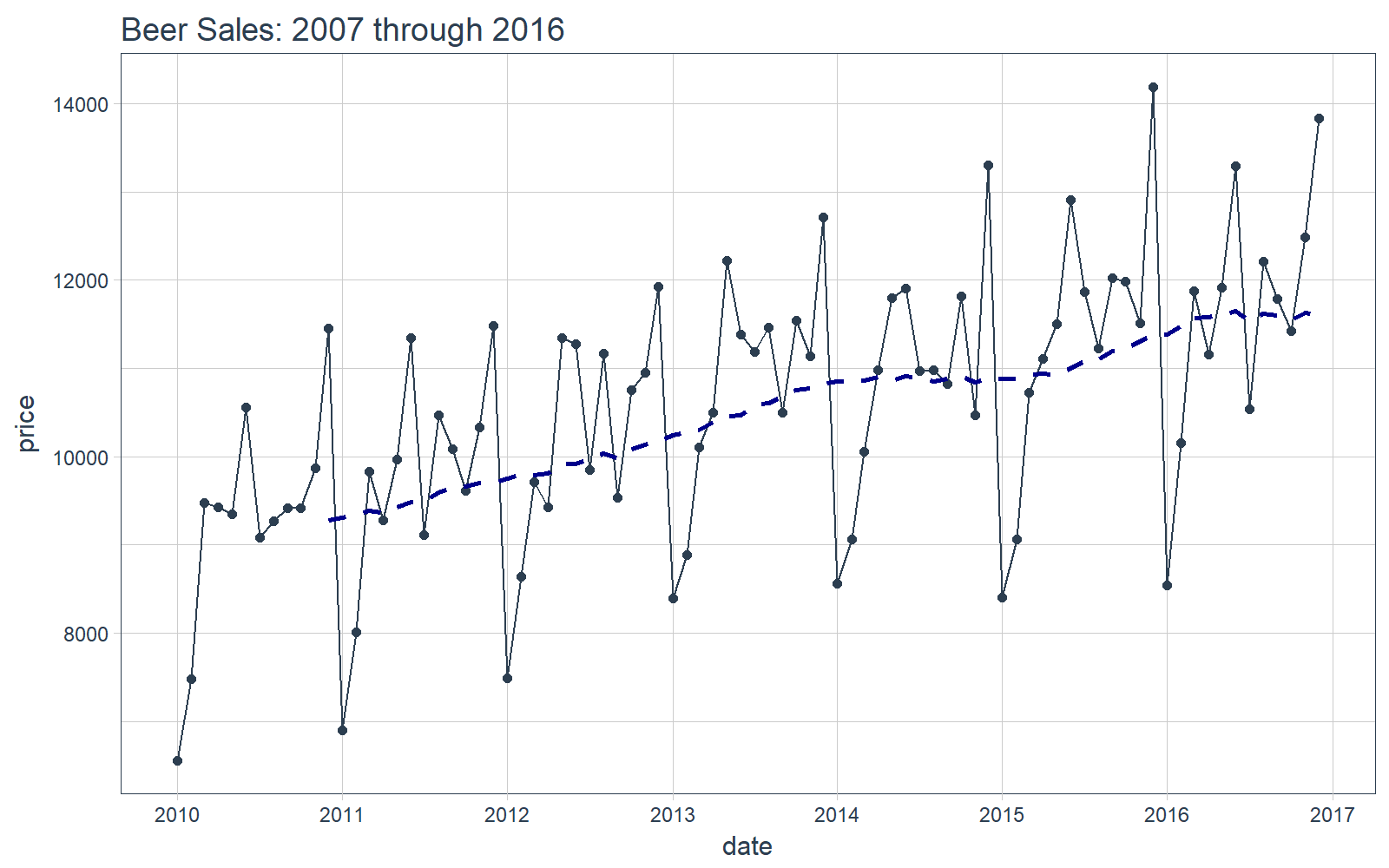
It’s a good idea to visualize the data so we know what we’re working with. Visualization is particularly important for time series analysis and forecasting (as we see during time series machine learning). We’ll use tidyquant charting tools: mainly geom_ma(ma_fun = SMA, n = 12) to add a 12-period simple moving average to get an idea of the trend. We can also see there appears to be both trend (moving average is increasing in a relatively linear pattern) and some seasonality (peaks and troughs tend to occur at specific months).
# Plot Beer Sales
beer_sales_tbl %>%
    ggplot(aes(date, price)) +
    geom_line(col = palette_light()[1]) +
    geom_point(col = palette_light()[1]) +
    geom_ma(ma_fun = SMA, n = 12, size = 1) +
    theme_tq() +
    scale_x_date(date_breaks = "1 year", date_labels = "%Y") +
    labs(title = "Beer Sales: 2007 through 2016")
Now that you have a feel for the time series we’ll be working with today, let’s move onto the demo!
DEMO: Tidy forecasting with forecast + sweep
We’ll use the combination of forecast and sweep to perform tidy forecasting.
Key Insight:
Forecasting using the forecast package is a non-tidy process that involves ts class objects. We have seen this system before where we can “tidy” these objects. For the stats library, we have broom, which tidies models and predictions. For the forecast package we now have sweep, which tidies models and forecasts.
Objective: We’ll work through an ARIMA analysis to forecast the next 12 months of time series data.
Step 1: Create ts object
Use timetk::tk_ts() to convert from tbl to ts. From the previous post, we learned that this has two benefits:
- It’s a consistent method to convert to and from
ts.
- The ts-object contains a
timetk_idx (timetk index) as an attribute, which is the original time-based index.
Here’s how to convert. Remember that ts-objects are regular time series so we need to specify a start and a freq.
# Convert from tbl to ts
beer_sales_ts <- tk_ts(beer_sales_tbl, start = 2010, freq = 12)

beer_sales_ts
##        Jan   Feb   Mar   Apr   May   Jun   Jul   Aug   Sep   Oct
## 2010  6558  7481  9475  9424  9351 10552  9077  9273  9420  9413
## 2011  6901  8014  9833  9281  9967 11344  9106 10468 10085  9612
## 2012  7486  8641  9709  9423 11342 11274  9845 11163  9532 10754
## 2013  8395  8888 10109 10493 12217 11385 11186 11462 10494 11541
## 2014  8559  9061 10058 10979 11794 11906 10966 10981 10827 11815
## 2015  8398  9061 10720 11105 11505 12903 11866 11223 12023 11986
## 2016  8540 10158 11879 11155 11916 13291 10540 12212 11786 11424
##        Nov   Dec
## 2010  9866 11455
## 2011 10328 11483
## 2012 10953 11922
## 2013 11139 12709
## 2014 10466 13303
## 2015 11510 14190
## 2016 12482 13832
We can check that the ts-object has a timetk_idx.
# Check that ts-object has a timetk index
has_timetk_idx(beer_sales_ts)
## [1] TRUE
Great. This will be important when we use sw_sweep() later. Next, we’ll model using ARIMA.
Step 2A: Model using ARIMA
We can use the auto.arima() function from the forecast package to model the time series.
# Model using auto.arima
fit_arima <- auto.arima(beer_sales_ts)

fit_arima
## Series: beer_sales_ts
## ARIMA(3,0,0)(1,1,0)[12] with drift
##
## Coefficients:
##           ar1     ar2     ar3     sar1    drift
##       -0.2498  0.1079  0.6210  -0.2817  32.1157
## s.e.   0.0933  0.0982  0.0925   0.1333   5.8882
##
## sigma^2 estimated as 175282:  log likelihood=-535.49
## AIC=1082.97   AICc=1084.27   BIC=1096.63
Step 2B: Tidy the Model
Like broom tidies the stats package, we can use sweep functions to tidy the ARIMA model. Let’s examine three tidiers, which enable tidy model evaluation:
sw_tidy(): Used to retrieve the model coefficientssw_glance(): Used to retrieve model description and training set accuracy metricssw_augment(): Used to get model residuals
sw_tidy
The sw_tidy() function returns the model coefficients in a tibble (tidy data frame).
# sw_tidy - Get model coefficients
sw_tidy(fit_arima)
## # A tibble: 5 x 2
##    term   estimate
##   <chr>      <dbl>
## 1   ar1 -0.2497937
## 2   ar2  0.1079269
## 3   ar3  0.6210345
## 4  sar1 -0.2816877
## 5 drift 32.1157478
sw_glance
The sw_glance() function returns the training set accuracy measures in a tibble (tidy data frame). We use glimpse to aid in quickly reviewing the model metrics.
# sw_glance - Get model description and training set accuracy measures
sw_glance(fit_arima) %>%
    glimpse()
## Observations: 1
## Variables: 12
## $ model.desc <chr> "ARIMA(3,0,0)(1,1,0)[12] with drift"
## $ sigma      <dbl> 418.6665
## $ logLik     <dbl> -535.4873
## $ AIC        <dbl> 1082.975
## $ BIC        <dbl> 1096.635
## $ ME         <dbl> 1.189875
## $ RMSE       <dbl> 373.9091
## $ MAE        <dbl> 271.7068
## $ MPE        <dbl> -0.06716239
## $ MAPE       <dbl> 2.526077
## $ MASE       <dbl> 0.4989005
## $ ACF1       <dbl> 0.02215405
sw_augment
The sw_augument() function helps with model evaluation. We get the “.actual”, “.fitted” and “.resid” columns, which are useful in evaluating the model against the training data. Note that we can pass timetk_idx = TRUE to return the original date index.
# sw_augment - get model residuals
sw_augment(fit_arima, timetk_idx = TRUE)
## # A tibble: 84 x 4
##         index .actual   .fitted    .resid
##        <date>   <dbl>     <dbl>     <dbl>
##  1 2010-01-01    6558  6551.474  6.525878
##  2 2010-02-01    7481  7473.583  7.416765
##  3 2010-03-01    9475  9465.621  9.378648
##  4 2010-04-01    9424  9414.704  9.295526
##  5 2010-05-01    9351  9341.810  9.190414
##  6 2010-06-01   10552 10541.641 10.359293
##  7 2010-07-01    9077  9068.148  8.852178
##  8 2010-08-01    9273  9263.984  9.016063
##  9 2010-09-01    9420  9410.869  9.130943
## 10 2010-10-01    9413  9403.908  9.091831
## # ... with 74 more rows
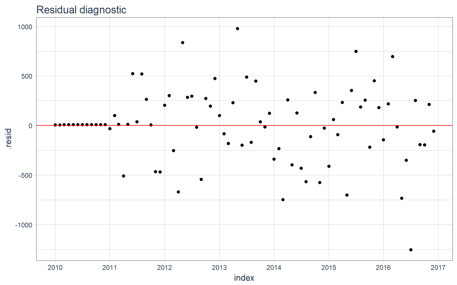
We can visualize the residual diagnostics for the training data to make sure there is no pattern leftover.
# Plotting residuals
sw_augment(fit_arima, timetk_idx = TRUE) %>%
    ggplot(aes(x = index, y = .resid)) +
    geom_point() +
    geom_hline(yintercept = 0, color = "red") +
    labs(title = "Residual diagnostic") +
    scale_x_date(date_breaks = "1 year", date_labels = "%Y") +
    theme_tq()
Step 3: Make a Forecast
Make a forecast using the forecast() function.
# Forecast next 12 months
fcast_arima <- forecast(fit_arima, h = 12)
One problem is the forecast output is not “tidy”. We need it in a data frame if we want to work with it using the tidyverse functionality. The class is “forecast”, which is a ts-based-object (its contents are ts-objects).
class(fcast_arima)
## [1] "forecast"
Step 4: Tidy the Forecast with sweep
We can use sw_sweep() to tidy the forecast output. As an added benefit, if the forecast-object has a timetk index, we can use it to return a date/datetime index as opposed to regular index from the ts-based-object.
First, let’s check if the forecast-object has a timetk index. Great. We can use the timetk_idx argument when we apply sw_sweep().
# Check if object has timetk index
has_timetk_idx(fcast_arima)
## [1] TRUE
Now, use sw_sweep() to tidy the forecast output. Internally it projects a future time series index based on “timetk_idx” that is an attribute (this all happens because we created the ts-object originally with tk_ts() in Step 1). Bottom Line: This means we can finally use dates with the forecast package (as opposed to the regularly spaced numeric index that the ts-system uses)!!!
# sw_sweep - tidies forecast output
fcast_tbl <- sw_sweep(fcast_arima, timetk_idx = TRUE)

fcast_tbl
## # A tibble: 96 x 7
##         index    key price lo.80 lo.95 hi.80 hi.95
##        <date>  <chr> <dbl> <dbl> <dbl> <dbl> <dbl>
##  1 2010-01-01 actual  6558    NA    NA    NA    NA
##  2 2010-02-01 actual  7481    NA    NA    NA    NA
##  3 2010-03-01 actual  9475    NA    NA    NA    NA
##  4 2010-04-01 actual  9424    NA    NA    NA    NA
##  5 2010-05-01 actual  9351    NA    NA    NA    NA
##  6 2010-06-01 actual 10552    NA    NA    NA    NA
##  7 2010-07-01 actual  9077    NA    NA    NA    NA
##  8 2010-08-01 actual  9273    NA    NA    NA    NA
##  9 2010-09-01 actual  9420    NA    NA    NA    NA
## 10 2010-10-01 actual  9413    NA    NA    NA    NA
## # ... with 86 more rows
Step 5: Compare Actuals vs Predictions
We can use tq_get() to retrieve the actual data. Note that we don’t have all of the data for comparison, but we can at least compare the first several months of actual values.
actuals_tbl <- tq_get("S4248SM144NCEN", get = "economic.data", from = "2017-01-01", to = "2017-12-31")
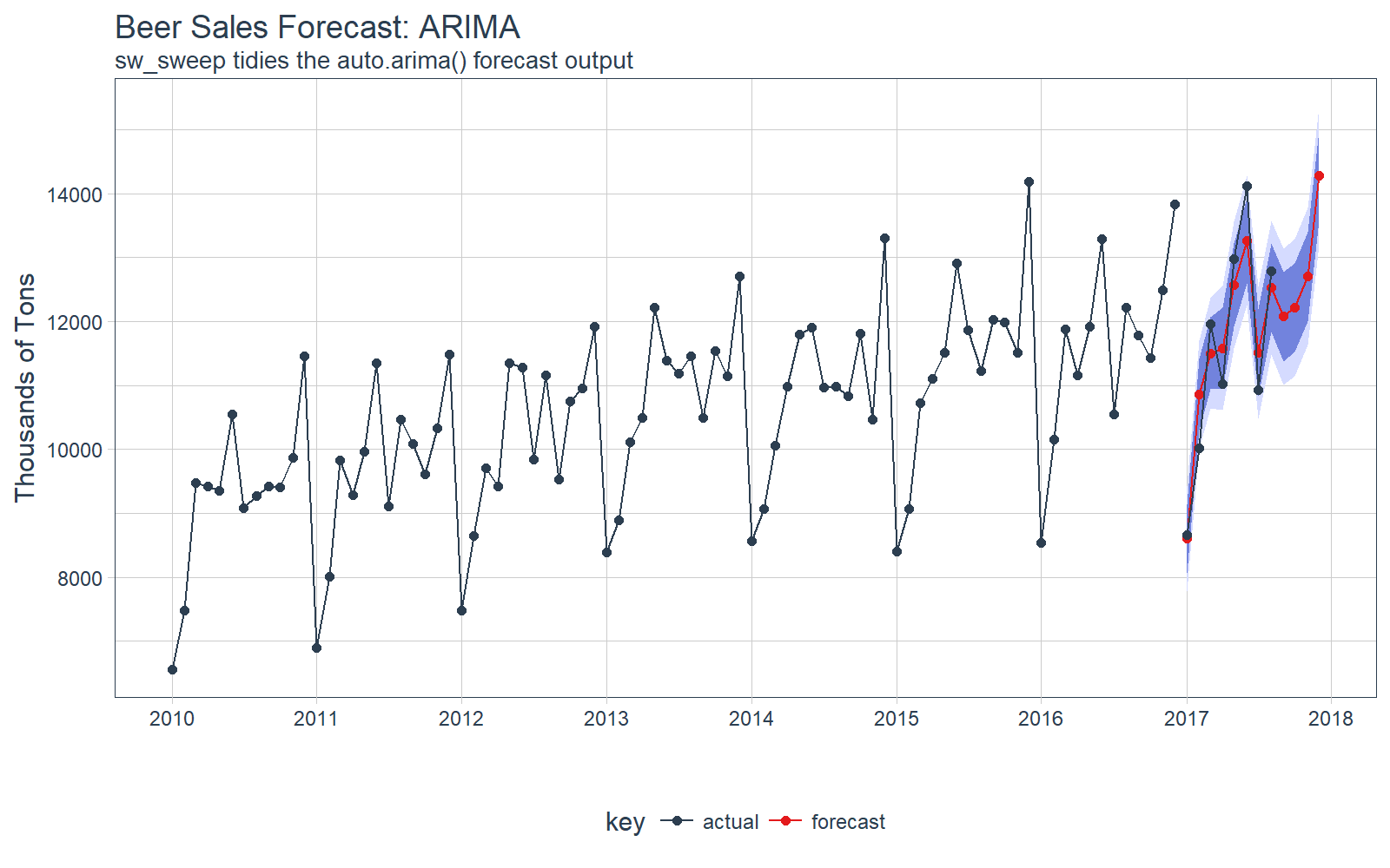
Notice that we have the entire forecast in a tibble. We can now more easily visualize the forecast.
# Visualize the forecast with ggplot
fcast_tbl %>%
    ggplot(aes(x = index, y = price, color = key)) +
    # 95% CI
    geom_ribbon(aes(ymin = lo.95, ymax = hi.95),
                fill = "#D5DBFF", color = NA, size = 0) +
    # 80% CI
    geom_ribbon(aes(ymin = lo.80, ymax = hi.80, fill = key),
                fill = "#596DD5", color = NA, size = 0, alpha = 0.8) +
    # Prediction
    geom_line() +
    geom_point() +
    # Actuals
    geom_line(aes(x = date, y = price), color = palette_light()[[1]], data = actuals_tbl) +
    geom_point(aes(x = date, y = price), color = palette_light()[[1]], data = actuals_tbl) +
    # Aesthetics
    labs(title = "Beer Sales Forecast: ARIMA", x = "", y = "Thousands of Tons",
         subtitle = "sw_sweep tidies the auto.arima() forecast output") +
    scale_x_date(date_breaks = "1 year", date_labels = "%Y") +
    scale_color_tq() +
    scale_fill_tq() +
    theme_tq()
We can investigate the error on our test set (actuals vs predictions).
# Investigate test error
error_tbl <- left_join(actuals_tbl, fcast_tbl, by = c("date" = "index")) %>%
    rename(actual = price.x, pred = price.y) %>%
    select(date, actual, pred) %>%
    mutate(
        error     = actual - pred,
        error_pct = error / actual
        )
error_tbl
## # A tibble: 8 x 5
##         date actual      pred      error    error_pct
##       <date>  <int>     <dbl>      <dbl>        <dbl>
## 1 2017-01-01   8664  8601.815   62.18469  0.007177365
## 2 2017-02-01  10017 10855.429 -838.42908 -0.083700617
## 3 2017-03-01  11960 11502.214  457.78622  0.038276439
## 4 2017-04-01  11019 11582.600 -563.59962 -0.051147982
## 5 2017-05-01  12971 12566.765  404.23491  0.031164514
## 6 2017-06-01  14113 13263.918  849.08191  0.060163106
## 7 2017-07-01  10928 11507.277 -579.27693 -0.053008504
## 8 2017-08-01  12788 12527.278  260.72219  0.020388035
And we can calculate a few residuals metrics. The MAPE error is approximately 4.3% from the actual value, which is slightly better than the simple linear regression from the timetk demo. Note that the RMSE is slighly worse.
# Calculate test error metrics
test_residuals <- error_tbl$error
test_error_pct <- error_tbl$error_pct * 100 # Percentage error

me   <- mean(test_residuals, na.rm=TRUE)
rmse <- mean(test_residuals^2, na.rm=TRUE)^0.5
mae  <- mean(abs(test_residuals), na.rm=TRUE)
mape <- mean(abs(test_error_pct), na.rm=TRUE)
mpe  <- mean(test_error_pct, na.rm=TRUE)

tibble(me, rmse, mae, mape, mpe) %>% glimpse()
## Observations: 1
## Variables: 5
## $ me   <dbl> 6.588034
## $ rmse <dbl> 561.4631
## $ mae  <dbl> 501.9144
## $ mape <dbl> 4.312832
## $ mpe  <dbl> -0.3835956
Next Steps
The sweep package is very useful for tidying the forecast package output. This demo showed some of the basics. Interested readers should check out the documentation, which goes into expanded detail on scaling analysis by groups and using multiple forecast models.
Announcements
We have a busy couple of weeks. In addition to Demo Week, we have:
DataTalk
On Thursday, October 26 at 7PM EST, Matt will be giving a FREE LIVE #DataTalk on Machine Learning for Recruitment and Reducing Employee Attrition. You can sign up for a reminder at the Experian Data Lab website.
EARL
On Friday, November 3rd, Matt will be presenting at the EARL Conference on HR Analytics: Using Machine Learning to Predict Employee Turnover.
Courses
Based on recent demand, we are considering offering application-specific machine learning courses for Data Scientists. The content will be business problems similar to our popular articles:
The student will learn from Business Science how to implement cutting edge data science to solve business problems. Please let us know if you are interested. You can leave comments as to what you would like to see at the bottom of the post in Disqus.
About Business Science
Business Science specializes in “ROI-driven data science”. Our focus is machine learning and data science in business applications. We help businesses that seek to add this competitive advantage but may not have the resources currently to implement predictive analytics. Business Science works with clients primarily in small to medium size businesses, guiding these organizations in expanding predictive analytics while executing on ROI generating projects. Visit the Business Science website or contact us to learn more!