Demo Week: class(Monday) <- tidyquant
Written by Matt Dancho

We’ve got an exciting week ahead of us at Business Science: we’re launching our first ever Business Science Demo Week. Every day this week we are demoing an R package: tidyquant (Monday), timetk (Tuesday), sweep (Wednesday), tibbletime (Thursday) and h2o (Friday)! That’s five packages in five days! We’ll give you intel on what you need to know about these packages to go from zero to hero. First up is tidyquant, our flagship package that’s useful for financial and time series analysis. Here we go!
Demo Week Demos:
Get The Best Resources In Data Science. Every Friday!
Sign up for our free "5 Topic Friday" Newsletter. Every week, I'll send you the five coolest topics in data science for business that I've found that week. These could be new R packages, free books, or just some fun to end the week on.
Sign Up For Five-Topic-Friday!
tidyquant: What’s It Used For?
Six reasons to use tidyquant:
-
Getting web data from Yahoo! Finance, FRED Database, Quandl and more
-
Tidy application of financial and time series functions from xts, zoo, quantmod, TTR and PerformanceAnalytics
-
Graphing: Beautiful themes and financial geoms (e.g. geom_ma)
-
Aggregating portfolios
-
Financial performance analysis and portfolio attribution metrics
-
Great base for financial and time series analysis: The tidyquant stack automatically loads the tidyverse and various time series / financial packages behind the scenes making it a great starting point for any financial or time series analysis
We’ll go over first two points in this demo. See the documentation for other topics.

Load Libraries
If you don’t have it installed, install tidyquant.
# Install libraries
install.packages("tidyquant")
Load the tidyquant package, which is all you need for the demo.
# Load libraries
library(tidyquant) # Loads tidyverse, financial pkgs, used to get and manipulate data
Getting data: tq_get
Use tq_get() to get data from the web. There’s a bunch of API’s it connects to including Yahoo! Finance, FRED Economic Database, Quandl, and more!
Getting Stock Prices (Yahoo! Finance)
Pass a vector of stock symbols to tq_get() setting get = "stock.prices". You can add from and to arguments to bound the daily stock prices to a window.
# Get Stock Prices from Yahoo! Finance

# Create a vector of stock symbols
FANG_symbols <- c("FB", "AMZN", "NFLX", "GOOG")

# Pass symbols to tq_get to get daily prices
FANG_data_d <- FANG_symbols %>%
    tq_get(get = "stock.prices", from = "2014-01-01", to = "2016-12-31")

# Show the result
FANG_data_d
## # A tibble: 3,024 x 8
##    symbol       date  open  high   low close   volume adjusted
##     <chr>     <date> <dbl> <dbl> <dbl> <dbl>    <dbl>    <dbl>
##  1     FB 2014-01-02 54.83 55.22 54.19 54.71 43195500    54.71
##  2     FB 2014-01-03 55.02 55.65 54.53 54.56 38246200    54.56
##  3     FB 2014-01-06 54.42 57.26 54.05 57.20 68852600    57.20
##  4     FB 2014-01-07 57.70 58.55 57.22 57.92 77207400    57.92
##  5     FB 2014-01-08 57.60 58.41 57.23 58.23 56682400    58.23
##  6     FB 2014-01-09 58.65 58.96 56.65 57.22 92253300    57.22
##  7     FB 2014-01-10 57.13 58.30 57.06 57.94 42449500    57.94
##  8     FB 2014-01-13 57.91 58.25 55.38 55.91 63010900    55.91
##  9     FB 2014-01-14 56.46 57.78 56.10 57.74 37503600    57.74
## 10     FB 2014-01-15 57.98 58.57 57.27 57.60 33663400    57.60
## # ... with 3,014 more rows
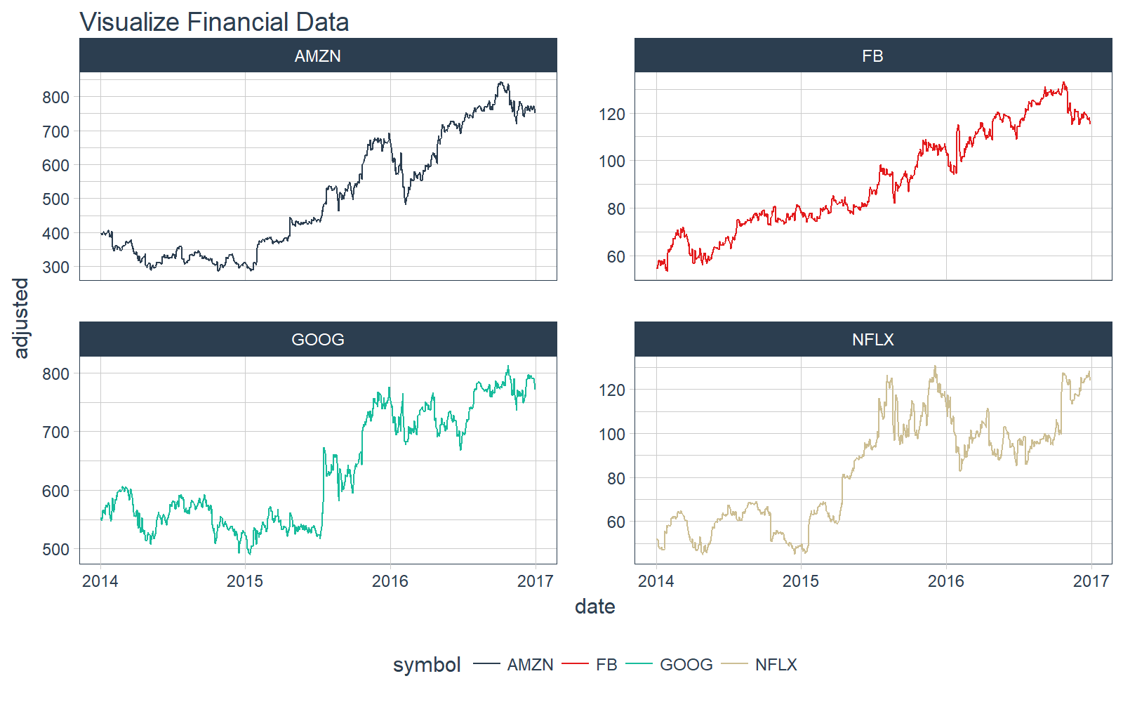
We can plot the results very easily using ggplot2. We’ll use tidyquant themes (theme_tq() and scale_color_tq()) for nice financial / business-ready graphs.
# Plot data
FANG_data_d %>%
    ggplot(aes(x = date, y = adjusted, color = symbol)) +
    geom_line() +
    facet_wrap(~ symbol, ncol = 2, scales = "free_y") +
    theme_tq() +
    scale_color_tq() +
    labs(title = "Visualize Financial Data")
Getting Economic Data (FRED)
This example comes from Deputy Chief Economist at Freddie Mac, Leonard Kieffer’s recent article A (TIDYQUANT)UM OF SOLACE. We’ll use tq_get() with the argument get = "economic.data" to retrieve data from the FRED economic database.
Pass a vector of FRED symbols to tq_get().
# Economic Data from the FRED

# Create a vector of FRED symbols
FRED_symbols <- c('ETOTALUSQ176N',    # All housing units
                  'EVACANTUSQ176N',   # Vacant
                  'EYRVACUSQ176N',    # Year-round vacant
                  'ERENTUSQ176N'      # Vacant for rent
)

# Pass symbols to tq_get to get economic data
FRED_data_m <- FRED_symbols %>%
    tq_get(get="economic.data", from = "2001-04-01")

# Show results
FRED_data_m
## # A tibble: 260 x 3
##           symbol       date  price
##            <chr>     <date>  <int>
##  1 ETOTALUSQ176N 2001-04-01 117786
##  2 ETOTALUSQ176N 2001-07-01 118216
##  3 ETOTALUSQ176N 2001-10-01 118635
##  4 ETOTALUSQ176N 2002-01-01 119061
##  5 ETOTALUSQ176N 2002-04-01 119483
##  6 ETOTALUSQ176N 2002-07-01 119909
##  7 ETOTALUSQ176N 2002-10-01 120350
##  8 ETOTALUSQ176N 2003-01-01 120792
##  9 ETOTALUSQ176N 2003-04-01 121233
## 10 ETOTALUSQ176N 2003-07-01 121682
## # ... with 250 more rows
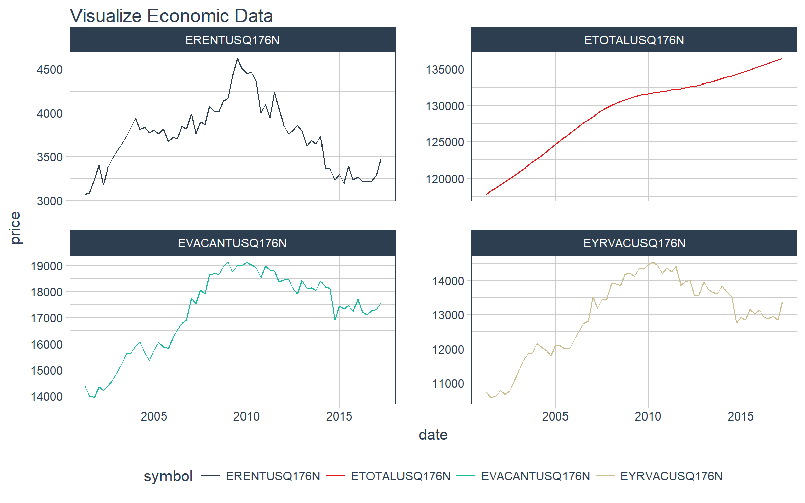
Like the financial data, we can plot the results very easily using ggplot2. We’ll again use tidyquant themes (theme_tq() and scale_color_tq()) for nice financial / business-ready graphs.
# Plot data
FRED_data_m %>%
    ggplot(aes(x = date, y = price, color = symbol)) +
    geom_line() +
    facet_wrap(~ symbol, ncol = 2, scales = "free_y") +
    theme_tq() +
    scale_color_tq() +
    labs(title = "Visualize Economic Data")
Mutating Data: tq_transmute and tq_mutate
The tq_transmute() and tq_mutate() functions are used to apply xts, zoo, and quantmod functions in a “tidy” way. We’ll jump right into how to use, but see below for Available Functions that are integrated into tidyquant.
tq_transmute
The difference between tq_transmute() and tq_mutate() is that tq_transmute() returns a new data frame whereas tq_mutate() grows the existing data frame width-wise (i.e. adds columns). The tq_transmute() function is most useful when periodicity changes the number of rows in the data.
Periodicity change with tq_transmute
Here’s an example of changing the periodicity from daily to monthly. You need to use tq_transmute() for this operation because the number of rows changes.
# Change periodicity from daily to monthly using to.period from xts
FANG_data_m <- FANG_data_d %>%
    group_by(symbol) %>%
    tq_transmute(
        select      = adjusted,
        mutate_fun  = to.period,
        period      = "months"
    )

FANG_data_m
## # A tibble: 144 x 3
## # Groups:   symbol [4]
##    symbol       date adjusted
##     <chr>     <date>    <dbl>
##  1     FB 2014-01-31    62.57
##  2     FB 2014-02-28    68.46
##  3     FB 2014-03-31    60.24
##  4     FB 2014-04-30    59.78
##  5     FB 2014-05-30    63.30
##  6     FB 2014-06-30    67.29
##  7     FB 2014-07-31    72.65
##  8     FB 2014-08-29    74.82
##  9     FB 2014-09-30    79.04
## 10     FB 2014-10-31    74.99
## # ... with 134 more rows
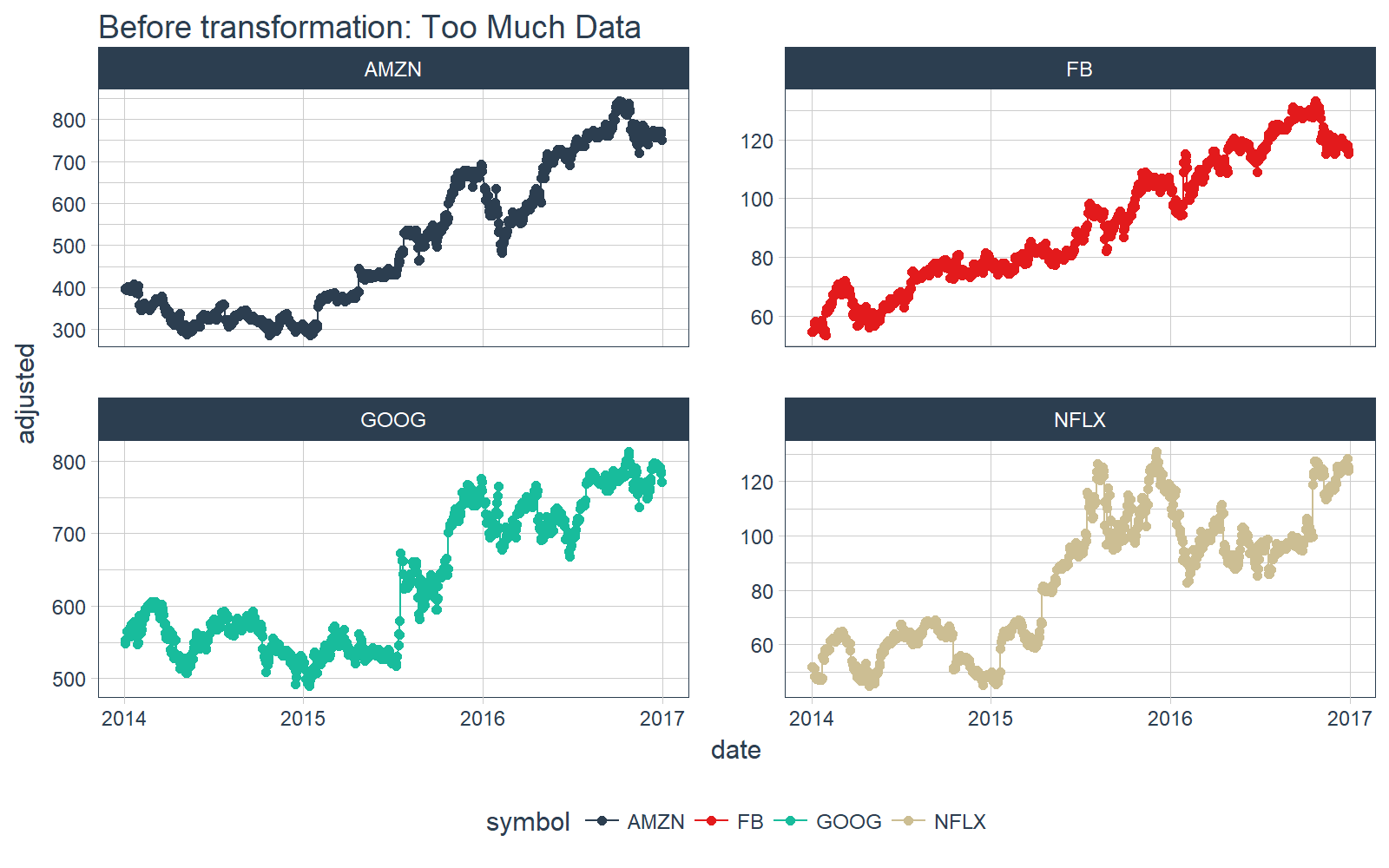
A simple reason you might want to perform a periodicity change is to reduce the amount of data. A couple notes:
- We use
theme_tq() and scale_color_tq() to create beautiful ggplots that are “business ready”
- If you need to change periodicity and do other time-based operations, pay attention on Thursday when we demo the new
tibbletime package… tibbletime takes time-based operations such as period changes to another level!!!
# Daily data
FANG_data_d %>%
    ggplot(aes(date, adjusted, color = symbol)) +
    geom_point() +
    geom_line() +
    facet_wrap(~ symbol, ncol = 2, scales = "free_y") +
    scale_color_tq() +
    theme_tq() +
    labs(title = "Before transformation: Too Much Data")
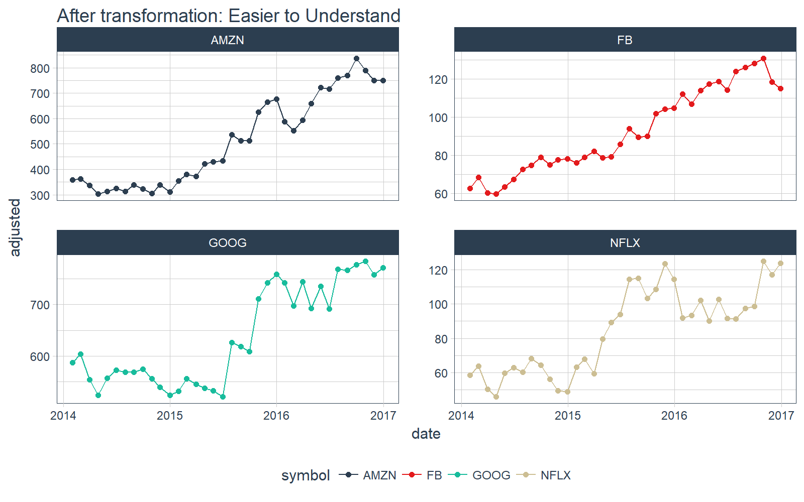
Much clearer when changed to a monthly scale via tq_transmute().
# Monthly data
FANG_data_m %>%
    ggplot(aes(date, adjusted, color = symbol)) +
    geom_point() +
    geom_line() +
    facet_wrap(~ symbol, ncol = 2, scales = "free_y") +
    scale_color_tq() +
    theme_tq() +
    labs(title = "After transformation: Easier to Understand")
tq_mutate
The tq_mutate() function returns the existing data frame column-binded with the output of the xts-based operation. Because of this, tq_mutate() is most useful when the number of columns returned is more than one (dplyr::mutate() doesn’t work in these situations).
Lags with tq_mutate
An example of this is with lag.xts. Typically we want more than one lag, which is where tq_mutate() shines. We’ll get the first five lags plus the original data.
# Lags - Get first 5 lags

# Pro Tip: Make the new column names first, then add to the `col_rename` arg
column_names <- paste0("lag", 1:5)

# First five lags are output for each group of symbols
FANG_data_d %>%
    select(symbol, date, adjusted) %>%
    group_by(symbol) %>%
    tq_mutate(
        select     = adjusted,
        mutate_fun = lag.xts,
        k          = 1:5,
        col_rename = column_names
    )
## # A tibble: 3,024 x 8
## # Groups:   symbol [4]
##    symbol       date adjusted  lag1  lag2  lag3  lag4  lag5
##     <chr>     <date>    <dbl> <dbl> <dbl> <dbl> <dbl> <dbl>
##  1     FB 2014-01-02    54.71    NA    NA    NA    NA    NA
##  2     FB 2014-01-03    54.56 54.71    NA    NA    NA    NA
##  3     FB 2014-01-06    57.20 54.56 54.71    NA    NA    NA
##  4     FB 2014-01-07    57.92 57.20 54.56 54.71    NA    NA
##  5     FB 2014-01-08    58.23 57.92 57.20 54.56 54.71    NA
##  6     FB 2014-01-09    57.22 58.23 57.92 57.20 54.56 54.71
##  7     FB 2014-01-10    57.94 57.22 58.23 57.92 57.20 54.56
##  8     FB 2014-01-13    55.91 57.94 57.22 58.23 57.92 57.20
##  9     FB 2014-01-14    57.74 55.91 57.94 57.22 58.23 57.92
## 10     FB 2014-01-15    57.60 57.74 55.91 57.94 57.22 58.23
## # ... with 3,014 more rows
Rolling functions with tq_mutate
Another example is applying a rolling function via the xts-based roll.apply(). Let’s apply the quantile() function to get rolling quantiles. We’ll specify the following arguments for each function:
tq_mutate arguments:
select = adjusted, We only want the adjusted column to be kept. We can leave blank or select a different subset of columns to be returned in addition to the output.mutate_fun = rollapply, This is the xts-based function that will be applied in a “tidy” way (to groups).
rollapply arguments:
width = 5, The width argument tells rollapply how many periods to use in the window calculation.by.column = FALSE, The rollapply() function defaults to applying functions to each column separately, however we want it to consider all columns in the operation.FUN = quantile: The quantile() function is applied in a rolling fashion.
quantile arguments:
probs = c(0, 0.025, ...), These are the probabilities that will be returned.na.rm = TRUE, Instructs quantile to remove NA values if present.
# Rolling quantile
FANG_data_d %>%
    select(symbol, date, adjusted) %>%
    group_by(symbol) %>%
    tq_mutate(
        select     = adjusted,
        mutate_fun = rollapply,
        width      = 5,
        by.column  = FALSE,
        FUN        = quantile,
        probs      = c(0, 0.025, 0.25, 0.5, 0.75, 0.975, 1),
        na.rm      = TRUE
    )
## # A tibble: 3,024 x 10
## # Groups:   symbol [4]
##    symbol       date adjusted   X0.  X2.5.  X25.  X50.  X75. X97.5.
##     <chr>     <date>    <dbl> <dbl>  <dbl> <dbl> <dbl> <dbl>  <dbl>
##  1     FB 2014-01-02    54.71    NA     NA    NA    NA    NA     NA
##  2     FB 2014-01-03    54.56    NA     NA    NA    NA    NA     NA
##  3     FB 2014-01-06    57.20    NA     NA    NA    NA    NA     NA
##  4     FB 2014-01-07    57.92    NA     NA    NA    NA    NA     NA
##  5     FB 2014-01-08    58.23 54.56 54.575 54.71 57.20 57.92 58.199
##  6     FB 2014-01-09    57.22 54.56 54.824 57.20 57.22 57.92 58.199
##  7     FB 2014-01-10    57.94 57.20 57.202 57.22 57.92 57.94 58.201
##  8     FB 2014-01-13    55.91 55.91 56.041 57.22 57.92 57.94 58.201
##  9     FB 2014-01-14    57.74 55.91 56.041 57.22 57.74 57.94 58.201
## 10     FB 2014-01-15    57.60 55.91 56.041 57.22 57.60 57.74 57.920
## # ... with 3,014 more rows, and 1 more variables: X100. <dbl>
Available Functions
We’ve just briefly touched on the xts-based functions that are integrated with tq_transmute and tq_mutate. There are a lot more xts-based functions that can be applied in a “tidy” way! Use tq_transmute_fun_options() to investigate other available functions.
# Available functions
# mutate_fun =
tq_transmute_fun_options()
## $zoo
##  [1] "rollapply"          "rollapplyr"         "rollmax"
##  [4] "rollmax.default"    "rollmaxr"           "rollmean"
##  [7] "rollmean.default"   "rollmeanr"          "rollmedian"
## [10] "rollmedian.default" "rollmedianr"        "rollsum"
## [13] "rollsum.default"    "rollsumr"
##
## $xts
##  [1] "apply.daily"     "apply.monthly"   "apply.quarterly"
##  [4] "apply.weekly"    "apply.yearly"    "diff.xts"
##  [7] "lag.xts"         "period.apply"    "period.max"
## [10] "period.min"      "period.prod"     "period.sum"
## [13] "periodicity"     "to.daily"        "to.hourly"
## [16] "to.minutes"      "to.minutes10"    "to.minutes15"
## [19] "to.minutes3"     "to.minutes30"    "to.minutes5"
## [22] "to.monthly"      "to.period"       "to.quarterly"
## [25] "to.weekly"       "to.yearly"       "to_period"
##
## $quantmod
##  [1] "allReturns"      "annualReturn"    "ClCl"
##  [4] "dailyReturn"     "Delt"            "HiCl"
##  [7] "Lag"             "LoCl"            "LoHi"
## [10] "monthlyReturn"   "Next"            "OpCl"
## [13] "OpHi"            "OpLo"            "OpOp"
## [16] "periodReturn"    "quarterlyReturn" "seriesAccel"
## [19] "seriesDecel"     "seriesDecr"      "seriesHi"
## [22] "seriesIncr"      "seriesLo"        "weeklyReturn"
## [25] "yearlyReturn"
##
## $TTR
##  [1] "adjRatios"          "ADX"                "ALMA"
##  [4] "aroon"              "ATR"                "BBands"
##  [7] "CCI"                "chaikinAD"          "chaikinVolatility"
## [10] "CLV"                "CMF"                "CMO"
## [13] "DEMA"               "DonchianChannel"    "DPO"
## [16] "DVI"                "EMA"                "EMV"
## [19] "EVWMA"              "GMMA"               "growth"
## [22] "HMA"                "KST"                "lags"
## [25] "MACD"               "MFI"                "momentum"
## [28] "OBV"                "PBands"             "ROC"
## [31] "rollSFM"            "RSI"                "runCor"
## [34] "runCov"             "runMAD"             "runMax"
## [37] "runMean"            "runMedian"          "runMin"
## [40] "runPercentRank"     "runSD"              "runSum"
## [43] "runVar"             "SAR"                "SMA"
## [46] "SMI"                "SNR"                "stoch"
## [49] "TDI"                "TRIX"               "ultimateOscillator"
## [52] "VHF"                "VMA"                "volatility"
## [55] "VWAP"               "VWMA"               "wilderSum"
## [58] "williamsAD"         "WMA"                "WPR"
## [61] "ZigZag"             "ZLEMA"
##
## $PerformanceAnalytics
## [1] "Return.annualized"        "Return.annualized.excess"
## [3] "Return.clean"             "Return.cumulative"
## [5] "Return.excess"            "Return.Geltner"
## [7] "zerofill"
Next Steps
We’ve only scratched the surface of tidyquant. There’s so much more to learn including tq_portfolio, tq_performance, charting capabilities, and more. Here are a few resources to help you along the way:
Announcements
We have a busy couple of weeks. In addition to Demo Week, we have:
DataTalk
On Thursday, October 26 at 7PM EST, Matt will be giving a FREE LIVE #DataTalk on Machine Learning for Recruitment and Reducing Employee Attrition. You can sign up for a reminder at the Experian Data Lab website.
EARL
On Friday, November 3rd, Matt will be presenting at the EARL Conference on HR Analytics: Using Machine Learning to Predict Employee Turnover.
Courses
Based on recent demand, we are considering offering application-specific machine learning courses for Data Scientists. The content will be business problems similar to our popular articles:
The student will learn from Business Science how to implement cutting edge data science to solve business problems. Please let us know if you are interested. You can leave comments as to what you would like to see at the bottom of the post in Disqus.
About Business Science
Business Science specializes in “ROI-driven data science”. Our focus is machine learning and data science in business applications. We help businesses that seek to add this competitive advantage but may not have the resources currently to implement predictive analytics. Business Science works with clients primarily in small to medium size businesses, guiding these organizations in expanding predictive analytics while executing on ROI generating projects. Visit the Business Science website or contact us to learn more!